

svm
写在前面
这是学习过程的一些tip,如有侵权,联系删除
linear_svm
from builtins import range
import numpy as np
from random import shuffle
from past.builtins import xrange


def svm_loss_naive(W, X, y, reg):
    """
    Structured SVM loss function, naive implementation (with loops).
    建立一个svm 损失函数, 本地执行(在循环基础上)
    Inputs have dimension D, there are C classes, and we operate on minibatches
    of N examples.
    输入我们对小批量进行操作的N个例子(D 维度, C类)。
    Inputs:
    - W: A numpy array of shape (D, C) containing weights.   包含权重的
    - X: A numpy array of shape (N, D) containing a minibatch of data.   包含小部分数据的
    - y: A numpy array of shape (N,) containing training labels; y[i] = c means
      that X[i] has label c, where 0 <= c < C.
    - reg: (float) regularization strength

    Returns a tuple of:
    - loss as single float
    - gradient with respect to weights W; an array of same shape as W
    """
    dW = np.zeros(W.shape)  # initialize the gradient as zero

    # compute the loss and the gradient
    num_classes = W.shape[1]  # 10
    num_train = X.shape[0]  # 500
    loss = 0.0
    for i in range(num_train):
        scores = X[i].dot(W)  # 评分函数 (1 *3073) * (3073 * 10) = 1 * 10  点积
        correct_class_score = scores[y[i]]  # 正确的类的得分, y[i] 第i个元素的标签标号
        for j in range(num_classes):  # 10个种类, 0 到 9遍历 scores
            if j == y[i]:  # 如果y[i] = j 那么就不处理,因为这个就是正确分类的得分
                continue
            margin = scores[j] - correct_class_score + 1  # note delta = 1, 一般delta都设置为1, 这个效果不错
            if margin > 0:  # max(0, margin)
                loss += margin  # 当得分margin 比 0大就加入损失值
                dW[:, j] += X[i]
                dW[:, y[i]] -= X[i]
    # Right now the loss is a sum over all training examples, but we want it
    # to be an average instead so we divide by num_train.
    loss /= num_train  # 要计算平均损失值,所以要除以总项数

    # Add regularization to the loss. 正则化损失
    loss += reg * np.sum(W * W)  # loss += reg * np.sum(np.square(W)) 这是最常用的正则化惩罚——L2 范式
    # reg 一般无法直接取得,需要进行交叉验证取得
    #############################################################################
    # TODO:                                                                     #
    # Compute the gradient of the loss function and store it dW.                #
    # Rather that first computing the loss and then computing the derivative,   #
    # it may be simpler to compute the derivative at the same time that the     #
    # loss is being computed. As a result you may need to modify some of the    #
    # code above to compute the gradient.                                       #
    #############################################################################
    # *****START OF YOUR CODE (DO NOT DELETE/MODIFY THIS LINE)*****
    # 求梯度
    dW /= (1.0 * num_train)
    dW += 2.0 * reg * W

    # *****END OF YOUR CODE (DO NOT DELETE/MODIFY THIS LINE)*****

    return loss, dW


def svm_loss_vectorized(W, X, y, reg):
    """
    Structured SVM loss function, vectorized implementation.

    Inputs and outputs are the same as svm_loss_naive.
    """
    loss = 0.0
    dW = np.zeros(W.shape)  # initialize the gradient as zero

    #############################################################################
    # TODO:                                                                     #
    # Implement a vectorized version of the structured SVM loss, storing the    #
    # result in loss.                                                           #
    #############################################################################
    # *****START OF YOUR CODE (DO NOT DELETE/MODIFY THIS LINE)*****

    num_train = X.shape[0]
    scores = X.dot(W)
    correct_class_score = scores[np.arange(num_train), y]  # different with scores[:, y]
    # 将每行的正确的类的分数添加进 correct_class_score
    margins = np.maximum(0, scores - correct_class_score[:, np.newaxis] + 1)
    # newaxis 为numpy数组添加一个维度, 这里相当于将一维数组转变为二维数组, 就变成 500 * 1的二维数组
    margins[np.arange(num_train), y] = 0
    # 将正确分类的分数置为0
    loss += np.sum(margins)  # 对margins 数组内的所有元素求和, 也就是完成数据损失的计算
    loss /= num_train  # 对数据损失和求平均
    loss += reg * np.sum(W * W)  # 添加正则化损失

    # *****END OF YOUR CODE (DO NOT DELETE/MODIFY THIS LINE)*****

    #############################################################################
    # TODO:                                                                     #
    # Implement a vectorized version of the gradient for the structured SVM     #
    # loss, storing the result in dW.                                           #
    #                                                                           #
    # Hint: Instead of computing the gradient from scratch, it may be easier    #
    # to reuse some of the intermediate values that you used to compute the     #
    # loss.                                                                     #
    #############################################################################
    # *****START OF YOUR CODE (DO NOT DELETE/MODIFY THIS LINE)*****

    margins[margins > 0] = 1.0
    num_to_loss = np.sum(margins, axis=1)

    margins[np.arange(num_train), y] = -num_to_loss
    dW = np.dot(X.T, margins) / num_train + 2 * reg * W

    # *****END OF YOUR CODE (DO NOT DELETE/MODIFY THIS LINE)*****

    return loss, dW
基于梯度的优化
一开始给出的权重矩阵取较小的数组,这一步叫做随机初始化,经过计算后得到一个数据一般来说没有什么有效表述(除非运气真的很好)
虽然得到的表示是没有任何意义的,但可以根据结果反馈取调整权重矩阵, 这个调整的过程就是训练的过程,也是机器学习学习的过程
训练的过程通过训练循环来完成:
(1)从训练集中抽取样本 X 及其对应的标签 y 或者说目标 ———— 输入输出的过程
(2)在X上运行网络(前向传播),得到预测值y_pred ———— 张量运算
(3)计算网络在这批数据上的损失,衡量y和y_pred间的距离———— 张量运算
(4)更新网络的所有权重,使网络在这批数据上的损失略微下降
第四步比较难,一般要改变W一个维度两次才能知道朝那个方向改变才会使网络在哲普数据上的损失值降低
比如原来这个维度的系数为0.3,一次前向传播,损失为0.5;当把系数置为0.35时,损失值可能为0.6,这反而增大了,
当系数为0.25时,损失值可能是 0.45。 这需要两步计算验证,但放到实际对象这种方案就不太适用,因为权重矩阵里可能由数千个系数
这会耗费很多运算资源和时间,这时候梯度可以很好的解决这个问题
网络中的所有运算都是可微,计算相对网络系数的梯度,然后向梯度反方向改变梯度,从而使损失值降低
数学基础
导数
连续:光滑函数f(X)= y, X的微小变化只会影响y的微小变化, 即带尖尖的不是连续函数
导数:当dx时的斜率即该点的导数
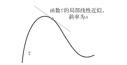
对于每个可微函数 f(x)(可微的意思是“可以被求导”。例如,光滑的连续函数可以被求导),
都存在一个导数函数 f'(x),将 x 的值映射为 f 在该点的局部线性近似的斜率。
梯度
当函数有多个参数的时候,我们称导数为偏导数。而梯度就是在每个维度上偏导数所形成的向量。
张量运算的导数就是梯度,这是导数的推广
一个输入向量 x、一个矩阵 W、一个目标 y 和一个损失函数 loss
用 W 来计算预测值 y_pred,然后计算损失,或者说预测值 y_pred 和目标 y 之间的距离。
y_pred = dot(W, x)
loss_value = loss(y_pred, y)
如果输入数据 x 和 y 保持不变,那么这可以看作将 W 映射到损失值的函数。
loss_value = f(W)
假设 W 的当前值为 W0。f 在 W0 点的导数是一个张量 gradient(f)(W0),其形状与 W 相同,
每个系数 gradient(f)(W0)[i, j] 表示改变 W0[i, j] 时 loss_value 变化的方向和大小。
张量 gradient(f)(W0) 是函数 f(W) = loss_value 在 W0 的导数。
对于一个函数 f(x),你可以通过将 x 向导数的反方向移动一小步来减小 f(x) 的值。同
样,对于张量的函数 f(W),你也可以通过将 W 向梯度的反方向移动来减小 f(W)
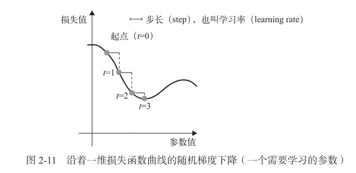
随机梯度下降(SDG)
对于一个可微的函数,其最小值位于其导数为0的点,
因此要找到函数的最小值,需要找到所有导数为0的点,并计算哪个是最小值(当然也有存在没有最小值的情况)比如 y=- x*x
小批量随机梯度下降
(1) 抽取训练样本 x 和对应目标 y 组成的数据批量。
(2) 在 x 上运行网络,得到预测值 y_pred。
(3) 计算网络在这批数据上的损失,用于衡量 y_pred 和 y 之间的距离。
(4) 计算损失相对于网络参数(权重)的梯度[一次反向传播(backward pass)]。
(5) 将参数沿着梯度的反方向移动一点,比如 W -= step * gradient,从而使这批数据
上的损失减小一点。
链式求导
根据微积分的知识,这种函数链可以利用下面这个恒等式进行求导,它称为链式法则(chainrule):
(f(g(x)))' = f'(g(x)) * g'(x)。
将链式法则应用于神经网络梯度值的计算,得到的算法叫作反向传播
(backpropagation,有时也叫反式微分,reverse-mode differentiation)。

 浙公网安备 33010602011771号