TessorFlow学习 之 神经网络的构建

 

---

 　　1.建立一个神经网络添加层

　　　　输入值、输入的大小、输出的大小和激励函数

　　　　学过神经网络的人看下面这个图就明白了，不懂的去看看我的另一篇博客

 

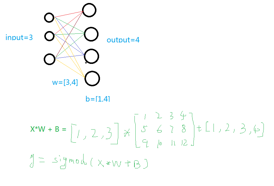
def add_layer(inputs , in_size , out_size , activate = None):
    Weights = tf.Variable(tf.random_normal([in_size,out_size]))#随机初始化
    baises  = tf.Variable(tf.zeros([1,out_size])+0.1)#可以随机但是不要初始化为0，都为固定值比随机好点
    y = tf.matmul(inputs, Weights) + baises #matmul:矩阵乘法，multipy:一般是数量的乘法
    if activate:
        y = activate(y)
    return y

 　　2.训练一个二次函数

import tensorflow as tf
import numpy as np

def add_layer(inputs , in_size , out_size , activate = None):
    Weights = tf.Variable(tf.random_normal([in_size,out_size]))#随机初始化
    baises  = tf.Variable(tf.zeros([1,out_size])+0.1)#可以随机但是不要初始化为0，都为固定值比随机好点
    y = tf.matmul(inputs, Weights) + baises #matmul:矩阵乘法，multipy:一般是数量的乘法
    if activate:
        y = activate(y)
    return y
if __name__ == '__main__':
    x_data = np.linspace(-1,1,300,dtype=np.float32)[:,np.newaxis]#创建-1,1的300个数，此时为一维矩阵，后面转化为二维矩阵===[1,2,3]-->>[[1,2,3]]
    noise = np.random.normal(0,0.05,x_data.shape).astype(np.float32)#噪声是(1,300)格式,0-0.05大小
    y_data = np.square(x_data) - 0.5 + noise #带有噪声的抛物线

    xs = tf.placeholder(tf.float32,[None,1]) #外界输入数据
    ys = tf.placeholder(tf.float32,[None,1])

    l1 = add_layer(xs,1,10,activate=tf.nn.relu)
    prediction = add_layer(l1,10,1,activate=None)

    loss = tf.reduce_mean(tf.reduce_sum(tf.square(ys - prediction),reduction_indices=[1]))#误差
    train_step = tf.train.GradientDescentOptimizer(0.1).minimize(loss)#对误差进行梯度优化，步伐为0.1

    sess = tf.Session()
    sess.run( tf.global_variables_initializer())
    for i in range(1000):
        sess.run(train_step, feed_dict={xs: x_data, ys: y_data})#训练
        if i%50 == 0:
            print(sess.run(loss, feed_dict={xs: x_data, ys: y_data}))#查看误差

 　　3.动态显示训练过程

　　　　显示的步骤程序之中部分进行说明，其它说明请看其它博客

import tensorflow as tf
import numpy as np
import matplotlib.pyplot as plt

def add_layer(inputs , in_size , out_size , activate = None):
    Weights = tf.Variable(tf.random_normal([in_size,out_size]))#随机初始化
    baises  = tf.Variable(tf.zeros([1,out_size])+0.1)#可以随机但是不要初始化为0，都为固定值比随机好点
    y = tf.matmul(inputs, Weights) + baises #matmul:矩阵乘法，multipy:一般是数量的乘法
    if activate:
        y = activate(y)
    return y
if __name__ == '__main__':
    x_data = np.linspace(-1,1,300,dtype=np.float32)[:,np.newaxis]#创建-1,1的300个数，此时为一维矩阵，后面转化为二维矩阵===[1,2,3]-->>[[1,2,3]]
    noise = np.random.normal(0,0.05,x_data.shape).astype(np.float32)#噪声是(1,300)格式,0-0.05大小
    y_data = np.square(x_data) - 0.5 + noise #带有噪声的抛物线
    fig = plt.figure('show_data')# figure("data")指定图表名称
    ax = fig.add_subplot(111)
    ax.scatter(x_data,y_data)
    plt.ion()
    plt.show()
    xs = tf.placeholder(tf.float32,[None,1]) #外界输入数据
    ys = tf.placeholder(tf.float32,[None,1])

    l1 = add_layer(xs,1,10,activate=tf.nn.relu)
    prediction = add_layer(l1,10,1,activate=None)

    loss = tf.reduce_mean(tf.reduce_sum(tf.square(ys - prediction),reduction_indices=[1]))#误差
    train_step = tf.train.GradientDescentOptimizer(0.1).minimize(loss)#对误差进行梯度优化，步伐为0.1

    sess = tf.Session()
    sess.run( tf.global_variables_initializer())
    for i in range(1000):
        sess.run(train_step, feed_dict={xs: x_data, ys: y_data})#训练
        if i%50 == 0:
            try:
                ax.lines.remove(lines[0])
            except Exception:
                pass
            prediction_value = sess.run(prediction, feed_dict={xs: x_data})
            lines = ax.plot(x_data,prediction_value,"r",lw = 3)
            print(sess.run(loss, feed_dict={xs: x_data, ys: y_data}))#查看误差
            plt.pause(2)
    while True:
        plt.pause(0.01)

 

 

　　 4.TensorBoard整体结构化显示

 

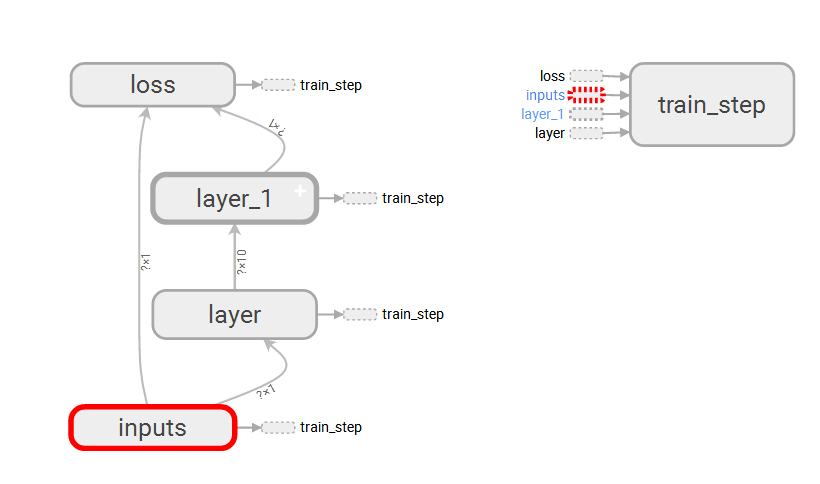
　　　　A.利用with tf.name_scope("name")创建大结构、利用函数的name="name"去创建小结构：tf.placeholder(tf.float32,[None,1],name="x_data")

　　　　B.利用writer = tf.summary.FileWriter("G:/test/",graph=sess.graph)创建一个graph文件

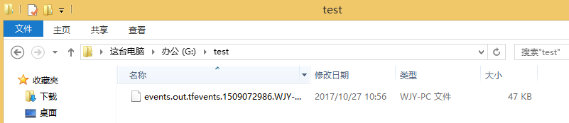
　　　　C.利用TessorBoard去执行这个文件

　　　　　　这里得注意--->>>首先到你存放文件的上一个目录--->>然后再去运行这个文件

　　　　　　tensorboard  --logdir=test

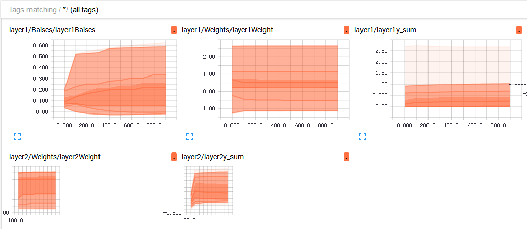
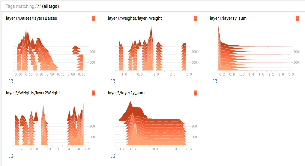
 　　5.TensorBoard局部结构化显示　　

　　　　　　A. tf.summary.histogram(layer_name+"Weight",Weights)：直方图显示

　　　　 

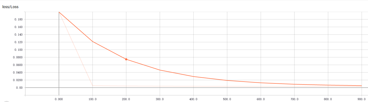
　　　　 B.  tf.summary.scalar("Loss",loss):折线图显示，loss的走向决定你的网络训练的好坏，至关重要一点

　　　　　  C.初始化与运行设定的图表

merge = tf.summary.merge_all()#合并图表
writer = tf.summary.FileWriter("G:/test/",graph=sess.graph)#写进文件
result = sess.run(merge,feed_dict={xs:x_data,ys:y_data})#运行打包的图表merge
writer.add_summary(result,i)#写入文件，并且单步长50

　　　　 完整代码及显示效果：

import tensorflow as tf
import numpy as np
import matplotlib.pyplot as plt

def add_layer(inputs , in_size , out_size , n_layer = 1 , activate = None):
    layer_name = "layer" + str(n_layer)
    with tf.name_scope(layer_name):
        with tf.name_scope("Weights"):
            Weights = tf.Variable(tf.random_normal([in_size,out_size]),name="W")#随机初始化
            tf.summary.histogram(layer_name+"Weight",Weights)
        with tf.name_scope("Baises"):
            baises  = tf.Variable(tf.zeros([1,out_size])+0.1,name="B")#可以随机但是不要初始化为0，都为固定值比随机好点
            tf.summary.histogram(layer_name+"Baises",baises)
        y = tf.matmul(inputs, Weights) + baises #matmul:矩阵乘法，multipy:一般是数量的乘法
        if activate:
            y = activate(y)
        tf.summary.histogram(layer_name+"y_sum",y)
        return y
if __name__ == '__main__':
    x_data = np.linspace(-1,1,300,dtype=np.float32)[:,np.newaxis]#创建-1,1的300个数，此时为一维矩阵，后面转化为二维矩阵===[1,2,3]-->>[[1,2,3]]
    noise = np.random.normal(0,0.05,x_data.shape).astype(np.float32)#噪声是(1,300)格式,0-0.05大小
    y_data = np.square(x_data) - 0.5 + noise #带有噪声的抛物线
    fig = plt.figure('show_data')# figure("data")指定图表名称
    ax = fig.add_subplot(111)
    ax.scatter(x_data,y_data)
    plt.ion()
    plt.show()
    with tf.name_scope("inputs"):
        xs = tf.placeholder(tf.float32,[None,1],name="x_data") #外界输入数据
        ys = tf.placeholder(tf.float32,[None,1],name="y_data")
    l1 = add_layer(xs,1,10,n_layer=1,activate=tf.nn.relu)
    prediction = add_layer(l1,10,1,n_layer=2,activate=None)
    with tf.name_scope("loss"):
        loss = tf.reduce_mean(tf.reduce_sum(tf.square(ys - prediction),reduction_indices=[1]))#误差
        tf.summary.scalar("Loss",loss)
    with tf.name_scope("train_step"):
        train_step = tf.train.GradientDescentOptimizer(0.1).minimize(loss)#对误差进行梯度优化，步伐为0.1

    sess = tf.Session()
    merge = tf.summary.merge_all()#合并
    writer = tf.summary.FileWriter("G:/test/",graph=sess.graph)
    sess.run( tf.global_variables_initializer())
    for i in range(1000):
        sess.run(train_step, feed_dict={xs: x_data, ys: y_data})#训练
        if i%100 == 0:
            result = sess.run(merge,feed_dict={xs:x_data,ys:y_data})#运行打包的图表merge
            writer.add_summary(result,i)#写入文件，并且单步长50

注意： 假设你的py文件中写了tf的summary，并且存放在了此目录下“D:\test\logs” 调出cmd，cd到D:\test，然后输入tensorboard –logdir=logs。一定要cd到logs这个文件夹的上一级，其他会出现No graph definition files were found.问题。

 

 

主要参考莫凡大大：https://morvanzhou.github.io/

可视化出现问题了，参考这位大神：http://blog.csdn.net/fengying2016/article/details/54289931