
OpenCV计算机视觉学习(8)——图像轮廓处理(轮廓绘制,轮廓检索,轮廓填充,轮廓近似)
如果需要处理的原图及代码,请移步小编的GitHub地址
传送门:请点击我
如果点击有误:https://github.com/LeBron-Jian/ComputerVisionPractice
1,简单几何图像绘制
简单几何图像一般包括点,直线,矩阵,圆,椭圆,多边形等等。
下面学习一下 opencv对像素点的定义。图像的一个像素点有1或3个值,对灰度图像有一个灰度值,对彩色图像有3个值组成一个像素值,他们表现出不同的颜色。
其实有了点才能组成各种多边形,才能对多边形进行轮廓检测,所以下面先练习一下简单的几何图像绘制。
1.1 绘制直线
在OpenCV中,绘制直线使用的函数为 line() ,其函数原型如下:
def line(img, pt1, pt2, color, thickness=None, lineType=None, shift=None): # real signature unknown; restored from __doc__
    """
    line(img, pt1, pt2, color[, thickness[, lineType[, shift]]]) -> img
    .   @brief Draws a line segment connecting two points.
    .
    .   The function line draws the line segment between pt1 and pt2 points in the image. The line is
    .   clipped by the image boundaries. For non-antialiased lines with integer coordinates, the 8-connected
    .   or 4-connected Bresenham algorithm is used. Thick lines are drawn with rounding endings. Antialiased
    .   lines are drawn using Gaussian filtering.
    .
    .   @param img Image.
    .   @param pt1 First point of the line segment.
    .   @param pt2 Second point of the line segment.
    .   @param color Line color.
    .   @param thickness Line thickness.
    .   @param lineType Type of the line. See #LineTypes.
    .   @param shift Number of fractional bits in the point coordinates.
    """
    pass
可以看到这个函数主要接受参数为两个点的坐标,线的颜色(其中灰色图为一个数字,彩色图为1*3的数组)。
实践代码如下:
import cv2
import numpy as np
import matplotlib.pyplot as plt

# 生成一个空灰度图像
img1 = np.zeros((400, 400), np.uint8)
img1 = cv2.line(img1, (0, 0), (400, 400), 255, 5)

# 生成一个空彩色图像
img3 = np.zeros((400, 400, 3), np.uint8)
img3 = cv2.line(img3, (0, 0), (400, 400), (0, 255, 0), 5)

titles = ['gray line image', 'color line image']
res = [img1, img3]

for i in range(2):
    plt.subplot(1, 2, i+1)
    plt.imshow(res[i]), plt.title(titles[i])
    plt.xticks([]), plt.yticks([])

plt.show()
效果如下:
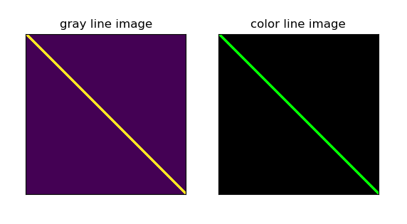
注意1:在这里再强调一下,由于cv和matplotlib的读取图像通道不同,导致灰度图和彩色图的颜色不一样,如果想分开看,可以直接使用cv2.imshow()。
注意2:绘制图像是在原图上绘制,这里我们写的是专门在原图上绘制,后面draw轮廓的话,可能需要 img.copy()了。不然我们的原图会存在画的轮廓。
1.2 绘制矩阵
在OpenCV中,绘制直线使用的函数为 rectangel() ,其函数原型如下:
def rectangle(img, pt1, pt2, color, thickness=None, lineType=None, shift=None): # real signature unknown; restored from __doc__
    """
    rectangle(img, pt1, pt2, color[, thickness[, lineType[, shift]]]) -> img
    .   @brief Draws a simple, thick, or filled up-right rectangle.
    .
    .   The function cv::rectangle draws a rectangle outline or a filled rectangle whose two opposite corners
    .   are pt1 and pt2.
    .
    .   @param img Image.
    .   @param pt1 Vertex of the rectangle.
    .   @param pt2 Vertex of the rectangle opposite to pt1 .
    .   @param color Rectangle color or brightness (grayscale image).
    .   @param thickness Thickness of lines that make up the rectangle. Negative values, like #FILLED,
    .   mean that the function has to draw a filled rectangle.
    .   @param lineType Type of the line. See #LineTypes
    .   @param shift Number of fractional bits in the point coordinates.


    rectangle(img, rec, color[, thickness[, lineType[, shift]]]) -> img
    .   @overload
    .
    .   use `rec` parameter as alternative specification of the drawn rectangle: `r.tl() and
    .   r.br()-Point(1,1)` are opposite corners
    """
    pass
参数解释
- 第一个参数img:img是原图
- 第二个参数pt1:(x,y)是矩阵的左上点坐标
- 第三个参数pt2:(x+w,y+h)是矩阵的右下点坐标
- 第四个参数color:(0,255,0)是画线对应的rgb颜色
- 第五个参数thickness:2是所画的线的宽度
cv2.rectangle(img, (10, 10), (390, 390), (255, 0, 0), 3),需要确定的就是矩形的两个点(左上角与右下角),颜色,线的类型(不设置就默认)。
代码如下:
import cv2
import numpy as np
import matplotlib.pyplot as plt
# 生成一个空灰度图像
img1 = np.zeros((400, 400), np.uint8)
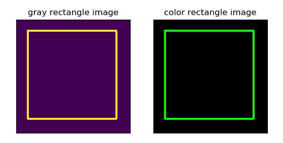
img1 = cv2.rectangle(img1, (40, 40), (350, 350), 255, 5)
# 生成一个空彩色图像
img3 = np.zeros((400, 400, 3), np.uint8)
img3 = cv2.rectangle(img3, (40, 40), (350, 350), (0, 255, 0), 5)
titles = ['gray rectangle image', 'color rectangle image']
res = [img1, img3]
for i in range(2):
plt.subplot(1, 2, i+1)
plt.imshow(res[i]), plt.title(titles[i])
plt.xticks([]), plt.yticks([])
plt.show()
效果如下:
1.3 绘制圆形
在OpenCV中,绘制直线使用的函数为 circle() ,其函数原型如下:
def circle(img, center, radius, color, thickness=None, lineType=None, shift=None): # real signature unknown; restored from __doc__
    """
    circle(img, center, radius, color[, thickness[, lineType[, shift]]]) -> img
    .   @brief Draws a circle.
    .
    .   The function cv::circle draws a simple or filled circle with a given center and radius.
    .   @param img Image where the circle is drawn.
    .   @param center Center of the circle.
    .   @param radius Radius of the circle.
    .   @param color Circle color.
    .   @param thickness Thickness of the circle outline, if positive. Negative values, like #FILLED,
    .   mean that a filled circle is to be drawn.
    .   @param lineType Type of the circle boundary. See #LineTypes
    .   @param shift Number of fractional bits in the coordinates of the center and in the radius value.
    """
    pass
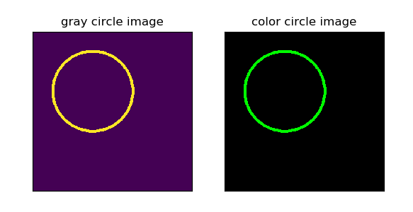
绘制圆形也简单,只需要确定圆心与半径即可。
实践代码如下:
import cv2
import numpy as np
import matplotlib.pyplot as plt

# 生成一个空灰度图像
img1 = np.zeros((400, 400), np.uint8)
img1 = cv2.circle(img1, (150, 150), 100, 255, 5)

# 生成一个空彩色图像
img3 = np.zeros((400, 400, 3), np.uint8)
img3 = cv2.circle(img3, (150, 150), 100, (0, 255, 0), 5)

titles = ['gray circle image', 'color circle image']
res = [img1, img3]

for i in range(2):
    plt.subplot(1, 2, i+1)
    plt.imshow(res[i]), plt.title(titles[i])
    plt.xticks([]), plt.yticks([])

plt.show()
效果如下:
1.4 绘制椭圆
在OpenCV中,绘制直线使用的函数为 ellipse() ,其函数原型如下:
def ellipse(img, center, axes, angle, startAngle, endAngle, color, thickness=None, lineType=None, shift=None): # real signature unknown; restored from __doc__
"""
ellipse(img, center, axes, angle, startAngle, endAngle, color[, thickness[, lineType[, shift]]]) -> img
. @brief Draws a simple or thick elliptic arc or fills an ellipse sector.
.
. The function cv::ellipse with more parameters draws an ellipse outline, a filled ellipse, an elliptic
. arc, or a filled ellipse sector. The drawing code uses general parametric form.
. A piecewise-linear curve is used to approximate the elliptic arc
. boundary. If you need more control of the ellipse rendering, you can retrieve the curve using
. #ellipse2Poly and then render it with #polylines or fill it with #fillPoly. If you use the first
. variant of the function and want to draw the whole ellipse, not an arc, pass `startAngle=0` and
. `endAngle=360`. If `startAngle` is greater than `endAngle`, they are swapped. The figure below explains
. the meaning of the parameters to draw the blue arc.
.
. 
.
. @param img Image.
. @param center Center of the ellipse.
. @param axes Half of the size of the ellipse main axes.
. @param angle Ellipse rotation angle in degrees.
. @param startAngle Starting angle of the elliptic arc in degrees.
. @param endAngle Ending angle of the elliptic arc in degrees.
. @param color Ellipse color.
. @param thickness Thickness of the ellipse arc outline, if positive. Otherwise, this indicates that
. a filled ellipse sector is to be drawn.
. @param lineType Type of the ellipse boundary. See #LineTypes
. @param shift Number of fractional bits in the coordinates of the center and values of axes.
ellipse(img, box, color[, thickness[, lineType]]) -> img
. @overload
. @param img Image.
. @param box Alternative ellipse representation via RotatedRect. This means that the function draws
. an ellipse inscribed in the rotated rectangle.
. @param color Ellipse color.
. @param thickness Thickness of the ellipse arc outline, if positive. Otherwise, this indicates that
. a filled ellipse sector is to be drawn.
. @param lineType Type of the ellipse boundary. See #LineTypes
"""
pass
这里解释一下参数:
- img:图像
- center:椭圆圆心坐标
- axes:轴的长度
- angle:偏转的角度
- start_angle:圆弧起始角的角度
- end_angle:圆弧终结角的角度
- color:线条的颜色
- thickness:线条的粗细程度
- line_type:线条的类型,详情见CVLINE的描述
- shift:圆心坐标点的数轴的精度
图像化如下:

实践代码如下:
import cv2
import numpy as np
import matplotlib.pyplot as plt
# 生成一个空灰度图像
img_origin1 = np.zeros((400, 400), np.uint8)
img_origin11 = img_origin1.copy()
# 参数依次是:图像,椭圆圆心坐标,轴的长度,偏转的角度, 圆弧起始角的角度,圆弧终结角的角度,线条的颜色,线条的粗细程度,线条的类型
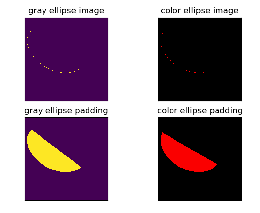
img1 = cv2.ellipse(img_origin1, (150, 150), (150, 100), 30, 10, 190, 250)
img11 = cv2.ellipse(img_origin11, (150, 150), (150, 100), 30, 10, 190, 250, -1)
# 生成一个空彩色图像
img_origin3 = np.zeros((400, 400, 3), np.uint8)
img_origin33 = img_origin3.copy()
# 注意最后一个参数 -1,表示对图像进行填充,默认是不填充的,如果去掉,只有椭圆轮廓了
img3 = cv2.ellipse(img_origin3, (150, 150), (150, 100), 30, 0, 180, 250)
img33 = cv2.ellipse(img_origin33, (150, 150), (150, 100), 30, 0, 180, 250, -1)
titles = ['gray ellipse image', 'color ellipse image', 'gray ellipse padding', 'color ellipse padding']
res = [img1, img3, img11, img33]
for i in range(4):
plt.subplot(2, 2, i+1)
plt.imshow(res[i]), plt.title(titles[i])
plt.xticks([]), plt.yticks([])
plt.show()
效果如下:
2,图像轮廓
图像轮廓可以简单认为成将连续的点(连着边界)连在一起的曲线,具有相同的颜色或者灰度。轮廓在形状分析和物体的检测和识别中很有用。
- 为了更加准确,要使用二值化图像。在寻找轮廓之前,要进行阈值化处理,或者Canny边界检测。
- 查找轮廓的函数会修改原始图像。如果你在找到轮廓之后还想使用原始图像的话,你应该将原始图像存储到其他变量中。
- 在OpenCV中,查找轮廓就像在黑色背景中超白色物体。你应该记住要找的物体应该是白色而背景应该是黑色。
2.1 cv2.findContours()函数
那么如何在一个二值化图像中查找轮廓呢?这里推荐使用函数cv2.findContours():
函数cv2.findContours()函数的原型为:
cv2.findContours(image, mode, method[, contours[, hierarchy[, offset ]]])
注意:opencv2返回两个值:contours:hierarchy。而opencv3会返回三个值,分别是img(图像), countours(轮廓,是一个列表,里面存贮着图像中所有的轮廓,每一个轮廓都是一个numpy数组,包含对象边界点(x, y)的坐标), hierarchy(轮廓的层析结构)。
函数参数:
第一个参数是寻找轮廓的图像,即输入图像;
第二个参数表示轮廓的检索模式,有四种(本文介绍的都是新的cv2接口):
- cv2.RETR_EXTERNAL: 表示只检测外轮廓
- cv2.RETR_LIST: 表示检测所有轮廓,检测的轮廓不建立等级关系,并将其保存到一条链表当中
- cv2.RETR_CCOMP :表示检测所有的轮廓,并将他们组织为两层:顶层是各部分的外部边界,第二次是空洞的边界
- cv2.RETR_TREE: 表示检测所有轮廓,并重构嵌套轮廓的整个层次,建立一个等级树结构的轮廓
第三个参数method为轮廓的近似办法
- cv2.CHAIN_APPROX_NONE:以Freeman链码的方式输出轮廓,所有其他方法输出多边形(顶点的序列)。存储所有的轮廓点,相邻的两个点的像素位置差不超过1,即max(abs(x1-x2),abs(y2-y1))==1
- cv2.CHAIN_APPROX_SIMPLE:压缩水平方向,垂直方向,对角线方向的元素,只保留该方向的终点坐标,例如一个矩形轮廓只需4个点来保存轮廓信息
- cv2.CHAIN_APPROX_TC89_L1,CV_CHAIN_APPROX_TC89_KCOS使用teh-Chinl chain 近似算法
这里轮廓的近似的两个方法我们可以从下面图看更加明显:
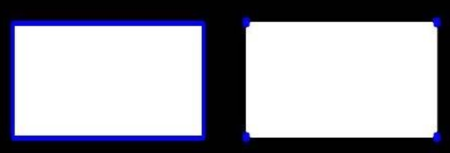
一个是输出所有轮廓(即所有顶点的序列),另一个函数只保留他们的终点部分。
函数返回值:
一般情况下,cv2.findContours()函数返回两个值,一个是轮廓本身,还有一个是每条轮廓对应的属性。当然特殊情况下返回三个值。即第一个是图像本身。
contour返回值
cv2.findContours()函数首先返回一个 list,list中每个元素都是图像中的一个轮廓,用numpy中的ndarray表示。这个概念非常重要,通过下面代码查看:
print (type(contours))
print (type(contours[0]))
print (len(contours))
'''
结果如下:
    <class 'list'>
    <class 'numpy.ndarray'>
    2
'''
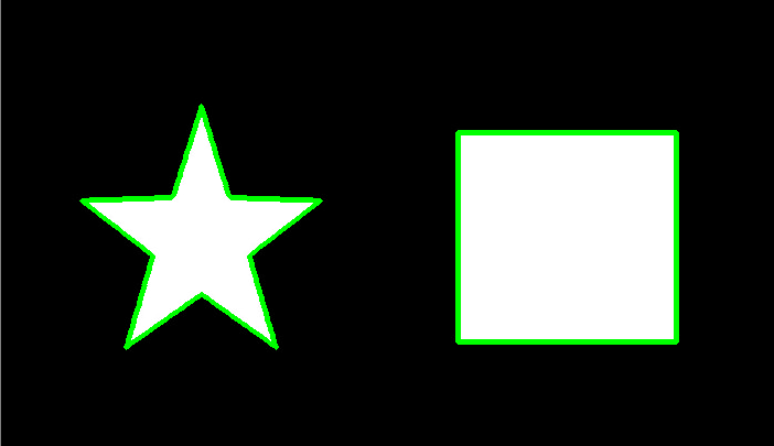
这里我们使用 contour.jpg 这幅图像举个例子,图如下:

通过上述图,我们会看到本例中有两条轮廓,一个是五角星的,一个是矩形的。每个轮廓是一个 ndarray,每个 ndarray是轮廓上的点的集合,并且打印出list的长度为2。
由于我们知道返回的轮廓有两个,因此可以通过:
cv2.drawContours(img,contours[0],0,(0,0,255),3)

cv2.drawContours(img,contours[1],0,(0,0,255),3)
分别绘制两个轮廓,同时通过:
print(len(contours[0]))
print(len(contours[1]))
'''
结果如下:
        4
        368
'''
输出两个轮廓中存储的点的个数,可以看出,第一个轮廓中只有四个元素,这是因为轮廓中并不是存储轮廓上所有的点,而是只存储可以用直线描述轮廓的点的个数,比如一个“正立”的矩形,只需要四个顶点就能描述轮廓了。而第二个轮廓却有368个元素,因为它是不规整的图像。
hiarachy返回值
此外,该函数还可返回一个可选的hiararchy结果,这是一个ndarray,其中的元素个数和轮廓个数相同,每个轮廓contours[i]对应4个hierarchy元素hierarchy[i][0] ~hierarchy[i][3],分别表示后一个轮廓、前一个轮廓、父轮廓、内嵌轮廓的索引编号,如果没有对应项,则该值为负数。
print (type(hierarchy))
print (hierarchy.ndim)
print (hierarchy[0].ndim)
print (hierarchy.shape)
'''
结果如下:
        <class 'numpy.ndarray'>
        3
        2
        (1, 2, 4)
'''
可以看出,hierachy本身包含两个ndarray,每个 ndarray对应一个轮廓,每个轮廓有四个属性。
完整代码如下:
import cv2

img = cv2.imread('contour.jpg')

gray = cv2.cvtColor(img, cv2.COLOR_BGR2GRAY)
ret, thresh = cv2.threshold(gray, 127, 255, cv2.THRESH_BINARY)
contours, hierarchy = cv2.findContours(thresh, cv2.RETR_TREE, cv2.CHAIN_APPROX_SIMPLE)

print (type(contours))
print (type(contours[0]))
print (len(contours))
'''
结果如下:
    <class 'list'>
    <class 'numpy.ndarray'>
    2
'''
print(len(contours[0]))
print(len(contours[1]))
'''
结果如下:
        4
        368
'''
print (type(hierarchy))
print (hierarchy.ndim)
print (hierarchy[0].ndim)
print (hierarchy.shape)
'''
结果如下:
        <class 'numpy.ndarray'>
        3
        2
        (1, 2, 4)
'''

# cv2.imshow('thresh', thresh)
# cv2.waitKey(0)
# cv2.destroyWindow('thresh')
2.2 cv2.drawContours()
OpenCV中通过 cv2.drawContours在图像上绘制轮廓。
下面看一下cv2.drawContours()函数:
cv2.drawContours(image, contours, contourIdx, color[,
thickness[, lineType[, hierarchy[, maxLevel[, offset ]]]]])
参数:
- 第一个参数是指明在哪幅图像上绘制轮廓;
- 第二个参数是轮廓本身,在Python中是一个list。
- 第三个参数指定绘制轮廓list中的哪条轮廓,如果是-1,则绘制其中的所有轮廓。后面的参数很简单。其中thickness表明轮廓线的宽度,如果是-1(cv2.FILLED),则为填充模式。绘制参数将在以后独立详细介绍。
下面看一个实例,在一幅图像上绘制所有的轮廓:
#_*_coding:utf-8_*_
import cv2
import numpy as np

img_path = 'contour.jpg'
img = cv2.imread(img_path)
img1 = img.copy()
img2 = img.copy()
img3 = img.copy()
imgray = cv2.cvtColor(img, cv2.COLOR_BGR2GRAY)
_, thresh = cv2.threshold(imgray, 127, 255, cv2.THRESH_BINARY)
contours, hierarchy= cv2.findContours(thresh, cv2.RETR_TREE, cv2.CHAIN_APPROX_SIMPLE)

# 绘制独立轮廓,如第四个轮廓
img1 = cv2.drawContours(img1, contours, -1, (0, 255, 0), 3)
# 如果指定绘制几个轮廓(确保数量在轮廓总数里面),就会只绘制指定数量的轮廓
img2 = cv2.drawContours(img2, contours, 1, (0, 255, 0), 3)
img3 = cv2.drawContours(img3, contours, 0, (0, 255, 0), 3)

res = np.hstack((img, img1, img2))
cv2.imshow('img', img3)
cv2.waitKey(0)
cv2.destroyAllWindows()
需要注意的是 cv2.findContours()函数接受的参数是二值图,即黑白的(不是灰度图),所以读取的图像先要转化成灰度图,再转化成二值图,后面两行代码分别是检测轮廓,绘制轮廓。
比如原图如下:

检测到的所有轮廓图如下(当指定绘制轮廓参数为 -1 ,默认绘制所有的轮廓):
当指定绘制轮廓的参数为 0的时候,则会找到索引为0的图像的轮廓如下:
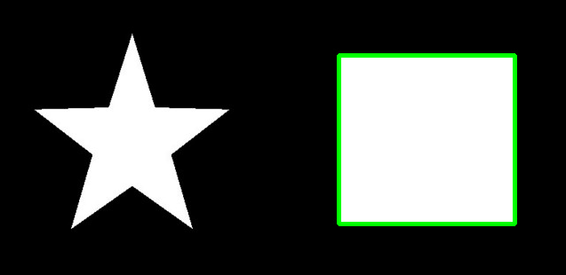
同理,当指定绘制轮廓的参数为 1的时候,则会找到索引为1的图像的轮廓如下:

注意:findcontours函数会“原地”修改输入的图像,所以我们需要copy图像,不然原图会变。。。。
2.3 cv2.boundingrect()函数
矩形边框(Bounding Rectangle)是说,用一个最小的矩形,把找到的形状包起来。还有一个带旋转的矩形,面积会更小。
首先介绍下cv2.boundingRect(img)这个函数,源码如下:
def boundingRect(array): # real signature unknown; restored from __doc__
    """
    boundingRect(array) -> retval
    .   @brief Calculates the up-right bounding rectangle of a point set or non-zero pixels of gray-scale image.
    .
    .   The function calculates and returns the minimal up-right bounding rectangle for the specified point set or
    .   non-zero pixels of gray-scale image.
    .
    .   @param array Input gray-scale image or 2D point set, stored in std::vector or Mat.
    """
    pass
解释一下参数的意义:img是一个二值图,也就是它的参数;返回四个值,分别是x,y,w,h( x,y是矩阵左上点的坐标,w,h是矩阵的宽和高);
用下面函数解释更加形象:
x, y, w, h = cv2.boudingrect(cnt) # 获得外接矩形

参数说明:x,y, w, h 分别表示外接矩形的x轴和y轴的坐标,以及矩形的宽和高, cnt表示输入的轮廓值
得到矩阵的坐标后,然后利用cv2.rectangle(img, (x,y), (x+w,y+h), (0,255,0), 2)画出矩行,我们前面有讲这个函数,这里不再赘述。
下面举个例子来看看如何找出不规则图像的外接矩阵,并画出其矩阵,首先图如下:
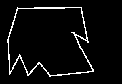
我们的目的是找出这个不规则图像的外接矩阵,并展示出来,代码如下:
#_*_coding:utf-8_*_
import cv2
import numpy as np

img_path = 'contour2.png'
img = cv2.imread(img_path)
img1 = img.copy()
img2 = img.copy()
imgray = cv2.cvtColor(img, cv2.COLOR_BGR2GRAY)
_, thresh = cv2.threshold(imgray, 127, 255, cv2.THRESH_BINARY)
contours, hierarchy= cv2.findContours(thresh, cv2.RETR_TREE, cv2.CHAIN_APPROX_NONE)
print('轮廓的总数为', len(contours))
# 轮廓的总数为 2

cnt = contours[0]
x, y, w, h = cv2.boundingRect(cnt)
img1 = cv2.rectangle(img1, (x,y), (x+w,y+h), (0, 255, 0), 2)

cv2.imshow('img', img1)
cv2.waitKey(0)
cv2.destroyAllWindows()
效果如下:

2.4 cv2.contourArea()
opencv中使用cv2.contourArea()来计算轮廓的面积。
首先介绍下cv2.contourArea(cnt, True)这个函数,源码如下:
def contourArea(contour, oriented=None): # real signature unknown; restored from __doc__
    """
    contourArea(contour[, oriented]) -> retval
    .   @brief Calculates a contour area.
    .
    .   The function computes a contour area. Similarly to moments , the area is computed using the Green
    .   formula. Thus, the returned area and the number of non-zero pixels, if you draw the contour using
    .   #drawContours or #fillPoly , can be different. Also, the function will most certainly give a wrong
    .   results for contours with self-intersections.
    .
    .   Example:
    .   @code
    .       vector<Point> contour;
    .       contour.push_back(Point2f(0, 0));
    .       contour.push_back(Point2f(10, 0));
    .       contour.push_back(Point2f(10, 10));
    .       contour.push_back(Point2f(5, 4));
    .
    .       double area0 = contourArea(contour);
    .       vector<Point> approx;
    .       approxPolyDP(contour, approx, 5, true);
    .       double area1 = contourArea(approx);
    .
    .       cout << "area0 =" << area0 << endl <<
    .               "area1 =" << area1 << endl <<
    .               "approx poly vertices" << approx.size() << endl;
    .   @endcode
    .   @param contour Input vector of 2D points (contour vertices), stored in std::vector or Mat.
    .   @param oriented Oriented area flag. If it is true, the function returns a signed area value,
    .   depending on the contour orientation (clockwise or counter-clockwise). Using this feature you can
    .   determine orientation of a contour by taking the sign of an area. By default, the parameter is
    .   false, which means that the absolute value is returned.
    """
    pass
参数含义如下:
- contour:表示某输入单个轮廓,为array
- oriented:表示某个方向上轮廓的面积值,这里指顺时针或者逆时针。若为True,该函数返回一个带符号的面积值,正负值取决于轮廓的方向(顺时针还是逆时针),若为False,表示以绝对值返回
面积的值与输入点的顺序有关,因为求的是按照点的顺序连接构成的图形的面积。
下面实践一下:
#_*_coding:utf-8_*_
import cv2
import numpy as np

img_path = 'contour2.png'
img = cv2.imread(img_path)
imgray = cv2.cvtColor(img, cv2.COLOR_BGR2GRAY)
_, thresh = cv2.threshold(imgray, 127, 255, cv2.THRESH_BINARY)
contours, hierarchy= cv2.findContours(thresh, cv2.RETR_TREE, cv2.CHAIN_APPROX_NONE)


cnt = contours[0]
# 求轮廓的面积
area = cv2.contourArea(cnt)
print(img.shape)  # (306, 453, 3)
print(area)  # 57436.5
# 也可以看轮廓面积与边界矩形比
x, y, w, h = cv2.boundingRect(cnt)
rect_area = w*h
extent = float(area) / rect_area
print('轮廓面积与边界矩形比为', extent)
# 轮廓面积与边界矩形比为 0.7800798598378357
2.5 cv2.arcLength()
opencv中使用cv2.arcLength()来计算轮廓的周长。
首先介绍下cv2.arcLength(cnt, True)这个函数,源码如下:
def arcLength(curve, closed): # real signature unknown; restored from __doc__
    """
    arcLength(curve, closed) -> retval
    .   @brief Calculates a contour perimeter or a curve length.
    .
    .   The function computes a curve length or a closed contour perimeter.
    .
    .   @param curve Input vector of 2D points, stored in std::vector or Mat.
    .   @param closed Flag indicating whether the curve is closed or not.
    """
    pass
参数含义如下:
- curve:输入的二维点集(轮廓顶点),可以是 vector或者Mat类型
- closed:用于指示曲线是否封闭
下面举个例子:
#_*_coding:utf-8_*_
import cv2
import numpy as np

img_path = 'contour2.png'
img = cv2.imread(img_path)
imgray = cv2.cvtColor(img, cv2.COLOR_BGR2GRAY)
_, thresh = cv2.threshold(imgray, 127, 255, cv2.THRESH_BINARY)
contours, hierarchy= cv2.findContours(thresh, cv2.RETR_TREE, cv2.CHAIN_APPROX_NONE)


cnt = contours[0]
# 求轮廓的周长
arcLength = cv2.arcLength(cnt, True)
print(img.shape)  # (306, 453, 3)
print(arcLength)  # 1265.9625457525253
2.6 cv2.approxPolyDP()
cv2.approxPolyDP()函数是轮廓近似函数,是opencv中对指定的点集进行多边形逼近的函数,其逼近的精度可通过参数设置。我们首先看一张图:
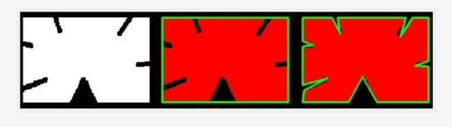
对于左边这张图,我们可以近似为中间和右边的这张图,具体如何近似呢?我们先不说,下面接着学。
下面看看cv2.approxPolyDP()函数的源码:
def approxPolyDP(curve, epsilon, closed, approxCurve=None): # real signature unknown; restored from __doc__
    """
    approxPolyDP(curve, epsilon, closed[, approxCurve]) -> approxCurve
    .   @brief Approximates a polygonal curve(s) with the specified precision.
    .
    .   The function cv::approxPolyDP approximates a curve or a polygon with another curve/polygon with less
    .   vertices so that the distance between them is less or equal to the specified precision. It uses the
    .   Douglas-Peucker algorithm <http://en.wikipedia.org/wiki/Ramer-Douglas-Peucker_algorithm>
    .
    .   @param curve Input vector of a 2D point stored in std::vector or Mat
    .   @param approxCurve Result of the approximation. The type should match the type of the input curve.
    .   @param epsilon Parameter specifying the approximation accuracy. This is the maximum distance
    .   between the original curve and its approximation.
    .   @param closed If true, the approximated curve is closed (its first and last vertices are
    .   connected). Otherwise, it is not closed.
    """
    pass
其参数含义:
- curve:表示输入的点集
- epslion:指定的精度,也即原始曲线与近似曲线之间的最大距离,不过这个值我们一般按照周长的大小进行比较
- close:若为True,则说明近似曲线为闭合的;反之,若为False,则断开
该函数采用的是道格拉斯—普克算法(Douglas-Peucker)来实现。该算法也以Douglas-Peucker 算法和迭代终点拟合算法为名。是将曲线近似表示为一系列点,并减少点的数量的一种算法。该算法的原始类型分别由乌尔斯-拉默(Urs Ramer)于 1972年以及大卫-道格拉斯(David Douglas)和托马斯普克(Thomas Peucker)于 1973年提出,并在之后的数十年中由其他学者完善。
经典的Douglas-Peucker 算法描述如下:
- 1,在曲线首位两点A, B之间连接一条直线AB,该直线为曲线的弦
- 2,得到曲线上离该直线段距离最大的点C,计算其与AB之间的距离d
- 3,比较该距离与预先给定的阈值 threshold 的大小,如果小于 threshold,则该直线段作为曲线的近似,该段曲线处理完毕
- 4,如果距离大于阈值,则用C将曲线分为两段AC和BC,并分别对两段取新进行1~3处理
- 5,当所有曲线都处理完毕后,依次连接各个分割点形成的折线,即可以作为曲线的近似
示意图如下:

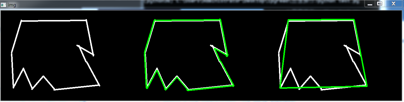
示例如下:
#_*_coding:utf-8_*_
import cv2
import numpy as np

img_path = 'contour2.png'
img = cv2.imread(img_path)
img1 = img.copy()
img2 = img.copy()
imgray = cv2.cvtColor(img, cv2.COLOR_BGR2GRAY)
_, thresh = cv2.threshold(imgray, 127, 255, cv2.THRESH_BINARY)
contours, hierarchy= cv2.findContours(thresh, cv2.RETR_TREE, cv2.CHAIN_APPROX_SIMPLE)

cnt = contours[0]
# 绘制独立轮廓,如第四个轮廓
img1 = cv2.drawContours(img1, [cnt], -1, (0, 255, 0), 3)

epsilon = 0.1*cv2.arcLength(cnt, True)
approx = cv2.approxPolyDP(cnt, epsilon, True)
img2 = cv2.drawContours(img2, [approx], -1, (0, 255, 0), 3)

res = np.hstack((img, img1, img2))
cv2.imshow('img', res)
cv2.waitKey(0)
cv2.destroyAllWindows()
效果如下:
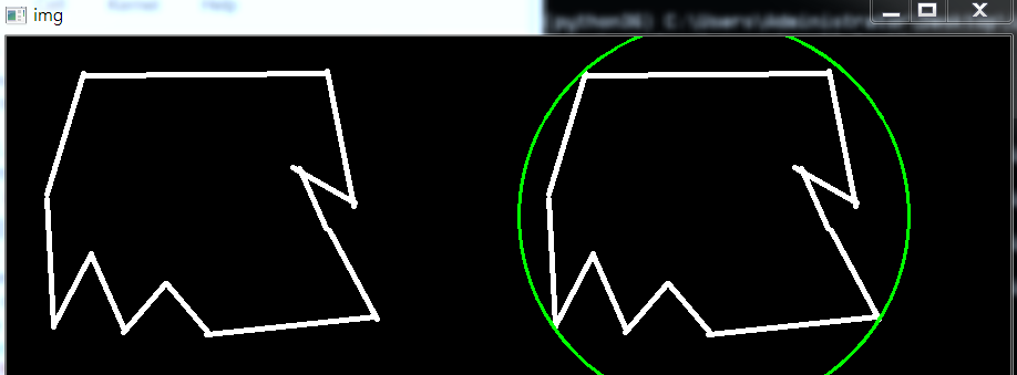
2.7 cv2.minEnclosingCircle()
在opencv中也可以实现轮廓的外接圆,它是函数cv2.minEnclosingCircle()。
下面我们看一下cv2.minEnclosingCircle()的源码:
def minEnclosingCircle(points): # real signature unknown; restored from __doc__
    """
    minEnclosingCircle(points) -> center, radius
    .   @brief Finds a circle of the minimum area enclosing a 2D point set.
    .
    .   The function finds the minimal enclosing circle of a 2D point set using an iterative algorithm.
    .
    .   @param points Input vector of 2D points, stored in std::vector\<\> or Mat
    .   @param center Output center of the circle.
    .   @param radius Output radius of the circle.
    """
    pass
参数意思也很明了,这里不再赘述。
实践代码如下:
#_*_coding:utf-8_*_
import cv2
import numpy as np

img_path = 'contour2.png'
img = cv2.imread(img_path)
img1 = img.copy()
imgray = cv2.cvtColor(img, cv2.COLOR_BGR2GRAY)
_, thresh = cv2.threshold(imgray, 127, 255, cv2.THRESH_BINARY)
contours, hierarchy= cv2.findContours(thresh, cv2.RETR_TREE, cv2.CHAIN_APPROX_NONE)


cnt = contours[0]
# 求轮廓的外接圆
(x, y), radius = cv2.minEnclosingCircle(cnt)
center = (int(x), int(y))
radius = int(radius)
img1 = cv2.circle(img1, center, radius, (0, 255, 0), 2)
res = np.hstack((img, img1))
cv2.imshow('img', res)
cv2.waitKey(0)
cv2.destroyAllWindows()
效果如下:
2.8 cv2.fillConvexPoly()与cv2.fillPoly()填充多边形
opencv中没有旋转矩形,也没有填充矩阵,但是它可以使用填充多边形函数 fillPoly()来填充。上面两个函数的区别就在于 fillConvexPoly() 画了一个凸多边形,这个函数要快得多,不过需要指定凸多边形的坐标。而fillPoly()则不仅可以填充凸多边形,任何单调多边形都可以填充。
cv2.fillConvexPoly()函数可以用来填充凸多边形,只需要提供凸多边形的顶点即可。
下面看看cv2.fillConvexPoly()函数的源码:
def fillConvexPoly(img, points, color, lineType=None, shift=None): # real signature unknown; restored from __doc__
    """
    fillConvexPoly(img, points, color[, lineType[, shift]]) -> img
    .   @brief Fills a convex polygon.
    .
    .   The function cv::fillConvexPoly draws a filled convex polygon. This function is much faster than the
    .   function #fillPoly . It can fill not only convex polygons but any monotonic polygon without
    .   self-intersections, that is, a polygon whose contour intersects every horizontal line (scan line)
    .   twice at the most (though, its top-most and/or the bottom edge could be horizontal).
    .
    .   @param img Image.
    .   @param points Polygon vertices.
    .   @param color Polygon color.
    .   @param lineType Type of the polygon boundaries. See #LineTypes
    .   @param shift Number of fractional bits in the vertex coordinates.
    """
    pass
示例如下:
#_*_coding:utf-8_*_
import cv2
import numpy as np

img = np.zeros((500, 500, 3), np.uint8)
triangle = np.array([[50, 50], [50, 400], [400, 450]])
cv2.fillConvexPoly(img, triangle, (0, 255, 0))
cv2.imshow('image', img)
cv2.waitKey(0)
cv2.destroyAllWindows()
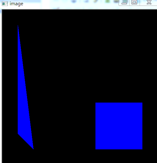
我们使用绿色填充,效果如下:

cv2.fillPoly()函数可以用来填充任意形状的图型.可以用来绘制多边形,工作中也经常使用非常多个边来近似的画一条曲线.cv2.fillPoly()函数可以一次填充多个图型。
下面看看cv2.fillPoly()函数的源码:
def fillPoly(img, pts, color, lineType=None, shift=None, offset=None): # real signature unknown; restored from __doc__
    """
    fillPoly(img, pts, color[, lineType[, shift[, offset]]]) -> img
    .   @brief Fills the area bounded by one or more polygons.
    .
    .   The function cv::fillPoly fills an area bounded by several polygonal contours. The function can fill
    .   complex areas, for example, areas with holes, contours with self-intersections (some of their
    .   parts), and so forth.
    .
    .   @param img Image.
    .   @param pts Array of polygons where each polygon is represented as an array of points.
    .   @param color Polygon color.
    .   @param lineType Type of the polygon boundaries. See #LineTypes
    .   @param shift Number of fractional bits in the vertex coordinates.
    .   @param offset Optional offset of all points of the contours.
    """
    pass
效果如下:
#_*_coding:utf-8_*_
import cv2
import numpy as np

img = np.zeros((500, 500, 3), np.uint8)
area1 = np.array([[50, 50], [50, 400], [100, 450]])
area2 = np.array([[300, 300],[450, 300], [450, 450], [300, 450]])
cv2.fillPoly(img, [area1, area2], (255, 0, 0))
cv2.imshow('image', img)
cv2.waitKey(0)
cv2.destroyAllWindows()
效果如下:
3,轮廓处理实战
下面举一个实际的例子来巩固一下学习的知识点。
问题是这样的,假设我相对这张图的左边面积做处理,我希望将其填充为白色(任何想要的颜色)。
也就是黑色圈外的颜色填充为白色,希望能完全利用上面学到的函数。
下面依次分析,首先对图像进行K-Means聚类,效果如下:

然后检测轮廓,这里尽量将所有的轮廓检测出来,如下:
然后对需要的轮廓进行填充,结果如下:
上图为最终的效果,代码如下:
import cv2
import numpy as np
import matplotlib.pyplot as plt


def show_image(img):
    cv2.imshow('image', img)
    cv2.waitKey(0)
    cv2.destroyAllWindows()


def image_processing(filename):
    img = cv2.imread(filename)
    img = cv2.resize(img, dsize=(100, 100))
    data = img.reshape((-1, 3))
    data = np.float32(data)
    # 定义中心(tyep, max_iter, epsilon)
    criteria = (cv2.TERM_CRITERIA_EPS + cv2.TERM_CRITERIA_MAX_ITER, 10, 1.0)
    # 设置标签
    flags = cv2.KMEANS_RANDOM_CENTERS
    # K-means 聚类,聚集成2类
    compactness, labels2, centers2 = cv2.kmeans(data, 2, None, criteria, 10, flags)

    # 2 类 图像转换回 uint8 二维类型
    centers2 = np.uint8(centers2)
    res2 = centers2[labels2.flatten()]
    dst2 = res2.reshape(img.shape)

    gray = cv2.cvtColor(dst2, cv2.COLOR_BGR2GRAY)
    _, thresh = cv2.threshold(gray, 127, 255, cv2.THRESH_BINARY)
    contours, hierarchy = cv2.findContours(thresh, cv2.RETR_TREE, cv2.CHAIN_APPROX_SIMPLE)
    # 第一个参数是指明在哪副图像上绘制轮廓,第二个参数是轮廓本身,在Python中是list
    # 第三个参数指定绘制轮廓list中那条轮廓,如果是-1,则绘制其中的所有轮廓。。
    # dst3 = cv2.drawContours(img, contours, -1, (0, 255, 0), 3)

    # show_image(dst3)
    for ind, contour in enumerate(contours):
        print('总共有几个轮廓:%s' % len(contours))

        # 其中x,y,w,h分布表示外接矩阵的x轴和y轴的坐标,以及矩阵的宽和高,contour表示输入的轮廓值
        x, y, w, h = cv2.boundingRect(contour)
        print(x, y, w, h)
        if w > 80 or h > 80:
            print(contours[ind])
            print(type(contours[ind]), contours[ind].shape)
            # cv2.fillConvexPoly()函数可以用来填充凸多边形,只需要提供凸多边形的顶点即可。
            cv2.fillConvexPoly(img, contours[ind], (255, 255, 255))
    show_image(img)

    # # 用来正常显示中文标签
    # plt.rcParams['font.sans-serif'] = ['SimHei']
    #
    # # 显示图形
    # titles = [u'原图', u'聚类图像 K=2']
    # images = [img,  dst2]
    # for i in range(len(images)):
    #     plt.subplot(1, 2, i + 1), plt.imshow(images[i], 'gray')
    #     plt.title(titles[i])
    #     plt.xticks([]), plt.yticks([])
    # plt.show()


if __name__ == '__main__':
    filename1 = 'test.png'
    image_processing(filename)
openCV Contours详解:https://www.pianshen.com/article/5989350739/
参考文献:https://blog.csdn.net/hjxu2016/article/details/77833336
https://blog.csdn.net/sunny2038/article/details/12889059#(写的好)
https://www.cnblogs.com/Ph-one/p/12082692.html
博客园函数:https://www.cnblogs.com/Undo-self-blog/p/8438808.html#top
https://blog.csdn.net/on2way/article/details/46793911

 浙公网安备 33010602011771号