
Python numpy总结(3)——常用函数用法
关于Python Numpy库基础知识请参考博文:Python NumPy学习(1)——numpy概述
关于Python Numpy矩阵知识请参考博文:Python numpy学习(2)——矩阵的用法
1,np.ceil(x, y)
限制元素范围,进一法,即向上取整。
x 表示输入的数据 y float类型 表示每个元素的上限。
a = np.array([-1.7, -1.5, -0.2, 0.2, 1.5, 1.7, 2.0])
np.ceil(a)

#  array([-1., -1., -0.,  1.,  2.,  2.,  2.])
2,np.random.permutation(x)
随机生成一个排列或返回一个 range,如果x 是一个多维数组,则只会沿着它的第一个索引进行混洗。
import numpy as np

shuffle_index = np.random.permutation(60000)
X_train, y_train = X_train[shuffle_index], y_train[shuffle_index]
函数np.random.permutation和np.random.shuffle用法的区别
函数shuffle与permutation都是对原来的数组进行重新洗牌(即随机打乱原来的元素顺序);区别在于shuffle直接在原来的数组上进行操作,改变原来数组的顺序,无返回值。而permutation不直接在原来的数组上进行操作,而是返回一个新的打乱顺序的数组,并不改变原来的数组。
示例:
a = np.arange(12)
print('origin a ',a)
np.random.shuffle(a)
print('shuffle a ',a)
print('\n')
a = np.arange(12)
print('origin a ',a)
b = np.random.permutation(a)
print('permutation b ',b)
print('deal with  a ',a)

'''
origin a  [ 0  1  2  3  4  5  6  7  8  9 10 11]
shuffle a  [ 5  8  2 10  7  3  0 11  6  9  4  1]


origin a  [ 0  1  2  3  4  5  6  7  8  9 10 11]
permutation b  [ 1 10  2 11  3  7  4  0  8  9  5  6]
deal with  a  [ 0  1  2  3  4  5  6  7  8  9 10 11]
'''
3,np.argmax()
返回沿轴的最大值的索引。
- a : array_like; 输入数组
- axis : int, optional; 默认情况下,索引是放在平面数组中,否则沿着指定的轴。
- out : array, optional; 如果提供,结果将被插入到这个数组中。它应该是适当的形状和dtype。
# some_digit_scores 内容
# array([[-311402.62954431, -363517.28355739, -446449.5306454 ,
#         -183226.61023518, -414337.15339485,  161855.74572176,
#         -452576.39616343, -471957.14962573, -518542.33997148,
#         -536774.63961222]])

np.argmax(some_digit_scores)
# Out
# 5
4,np.dot() 使用方法
(此函数参考:https://blog.csdn.net/skywalker1996/article/details/82462499)
np.dot() 函数主要有两个功能,向量点积和矩阵矩阵乘法,这里学习三种最常用的情况。
4.1 np.dot(a,b),其中a,b为一维的向量(a和b是 np.ndarray类型),此时做的是向量点积
import numpy as np

a = np.array([1, 2, 3, 4, 5])
b = np.array([6, 7, 8, 9, 10])
print(np.dot(a, b))  # 130
# 1*6 + 2*7 + 3*8 + 4*9 + 5*10
4.2 np.dot(a, b),其中a 为二维矩阵, b为一维向量,这里的b 会当做一维矩阵进行计算
the shape of a is (5, 5)
the shape of b is (5,)
[73 97 84 95 49]
the shape of np.dot(a,b) is (5,)
[[1 3 3 3 9]
 [1 4 8 6 8]
 [0 1 7 9 5]
 [9 8 4 7 6]
 [3 1 1 4 5]]
这里需要注意的是一维矩阵和一维向量的区别,一维向量的 shape是(5, ),而一维矩阵的 shape 是(5, 1),若这两个参数 a 和 b 都是一维向量则是计算的点积,但是当其中有一个是矩阵时(包括一维矩阵),dot便会进行矩阵乘法运算,同时若有个参数为向量,会自动转换为一维矩阵进行计算。
4.3 np.dot(a, b),其中a和b都是二维矩阵,此时 dot就是进行的矩阵乘法运算
import numpy as np

a = np.random.randint(0, 10, size=(5, 5))
b = np.random.randint(0, 10, size=(5, 3))
print("the shape of a is " + str(a.shape))
print("the shape of b is " + str(b.shape))
print(np.dot(a, b))
'''
the shape of a is (5, 5)
the shape of b is (5, 3)
[[120 162  56]
 [ 85 106  80]
 [146  99  94]
 [ 88  90  70]
 [130  87  80]]
 '''
5,np.linalg.inv()
计算矩阵的逆
- a : (..., M, M) array_like;被求逆的矩阵
X_b = np.c_[np.ones((100, 1)), X]  # add x0 = 1 to each instance

theta_best = np.linalg.inv(X_b.T.dot(X_b)).dot(X_b.T).dot(y)
6,np.ndarray.T()
计算矩阵的转置,如果self.ndim < 2 则返回它自身。
>>> x = np.array([[1.,2.],[3.,4.]])
>>> x
array([[ 1.,  2.],
       [ 3.,  4.]])
>>> x.T
array([[ 1.,  3.],
       [ 2.,  4.]])
>>> x = np.array([1.,2.,3.,4.])
>>> x
array([ 1.,  2.,  3.,  4.])
>>> x.T
array([ 1.,  2.,  3.,  4.])
7,Numpy增删一个值为1 的维度
(参考地址:https://www.jianshu.com/p/d1543cfaf737)
7.1 给2-d Array(H, W) 增加一个值为 1 的维度称为 3-d Array(H,W,1)
彩色图像 在 numpy中以 (H, W, C) 形状(channel-last)的 3-d Array 存储; 而 灰度图像 则以 (H, W) 形状的 2-d Array 存储, 经常需要为其增加一个值为 1 的维度, 成为 3-d Array(H, W, 1)。
import numpy as np

in:
a = np.ones((3,3))
print(a.shape)
b1 = np.expand_dims(a,2)
print(b1.shape)

out:
(2, 2)
(2, 2, 1)

note:
b2 = np.expand_dims(a, 0) # (1, 2, 2)
b3 = np.expand_dims(a, 1) # (2, 2, 1)
7.2 删去 d-d Array 中值为1 的维度
在显示,保存图像矩阵的时,往往需要删去值为1 的维度:
in:
a = np.ones((2,2,1))
print(a.shape)
b = np.squeeze(a)
print(b.shape)

out:
(2, 2, 1)
(2, 2)
8,np.random.normal()函数
np.random.normal()的意思是一个正态分布,normal这里是正态的意思。下面举一个例子:
random.normal(loc=0.5, scale=1e-2, size=shape)
解释一下:
1,参数 loc(float) :正态分布的均值,对应着这个分布的中心。loc=0说明这一个以Y轴为对称轴的正态分布。
2,参数 scale(float):正态分布的标准差,对应分布的宽度,scale越大,正态分布的曲线越矮胖,scale越小,曲线越高瘦。
3,参数size(int或者整数元组):输出的值赋在shape,默认为None。
9,np.linspace函数基本用法
在指定区间返回间隔均匀的样本 [start, stop]
- start : scalar;序列的起始值
- stop : scalar;序列的结束值
- num : int, optional;要生成的样本数量,默认为50个。
- endpoint : bool, optional;若为True则包括结束值,否则不包括结束值,即[start, stop)区间。默认为True。
- dtype : dtype, optional;输出数组的类型,若未给出则从输入数据推断类型。
X_new=np.linspace(-3, 3, 100).reshape(100, 1)
X_new_poly = poly_features.transform(X_new)
y_new = lin_reg.predict(X_new_poly)
plt.plot(X, y, "b.")
plt.plot(X_new, y_new, "r-", linewidth=2, label="Predictions")
plt.xlabel("$x_1$", fontsize=18)
plt.ylabel("$y$", rotation=0, fontsize=18)
plt.legend(loc="upper left", fontsize=14)
plt.axis([-3, 3, 0, 10])
save_fig("quadratic_predictions_plot")
plt.show()
10,Meshgrid函数基本用法
从坐标向量返回坐标矩阵。
理解:meshgrid函数用两个坐标轴上的点在平面上画网格。简单来说,meshgrid的作用适用于生成网格型数据,可以接受两个一维数组生成两个二维矩阵,对应两个数组中所有的(x, y)对
Meshgrid函数常用的场景有等高线绘制及机器学习中SVC超平面的绘制。
- x1, x2,..., xn : array_like;代表网格坐标的一维数组。
- indexing : {‘xy’, ‘ij’}, optional;输出的笛卡儿('xy',默认)或矩阵('ij')索引。
- sparse : bool, optional;如果为True则返回稀疏矩阵以减少内存,默认为False。
>>> nx, ny = (3, 2)
>>> x = np.linspace(0, 1, nx)
>>> y = np.linspace(0, 1, ny)
>>> xv, yv = np.meshgrid(x, y)
>>> xv
array([[ 0. ,  0.5,  1. ],
       [ 0. ,  0.5,  1. ]])
>>> yv
array([[ 0.,  0.,  0.],
       [ 1.,  1.,  1.]])
>>> xv, yv = np.meshgrid(x, y, sparse=True)  # make sparse output arrays
>>> xv
array([[ 0. ,  0.5,  1. ]])
>>> yv
array([[ 0.],
       [ 1.]])
11,norm()
矩阵或向量范数
- x : array_like;输入的数组,如果
axis是None,则x必须是1-D或2-D。 - ord : {non-zero int, inf, -inf, ‘fro’, ‘nuc’}, optional;范数的顺序,inf表示numpy的inf对象。
- axis : {int, 2-tuple of ints, None}, optional
- keepdims : bool, optional
t1a, t1b, t2a, t2b = -1, 3, -1.5, 1.5

# ignoring bias term
t1s = np.linspace(t1a, t1b, 500)
t2s = np.linspace(t2a, t2b, 500)
t1, t2 = np.meshgrid(t1s, t2s)
T = np.c_[t1.ravel(), t2.ravel()]
Xr = np.array([[-1, 1], [-0.3, -1], [1, 0.1]])
yr = 2 * Xr[:, :1] + 0.5 * Xr[:, 1:]

J = (1/len(Xr) * np.sum((T.dot(Xr.T) - yr.T)**2, axis=1)).reshape(t1.shape)

N1 = np.linalg.norm(T, ord=1, axis=1).reshape(t1.shape)
N2 = np.linalg.norm(T, ord=2, axis=1).reshape(t1.shape)

t_min_idx = np.unravel_index(np.argmin(J), J.shape)
t1_min, t2_min = t1[t_min_idx], t2[t_min_idx]

t_init = np.array([[0.25], [-1]])
12,unravel_index()
将平面索引或平面索引数组转换为坐标数组的元组
- indices : array_like;一个整数数组,其元素是索引到维数组dims的平坦版本中。
- dims : tuple of ints;用于分解索引的数组的形状。
- order : {‘C’, ‘F’}, optional;决定
indices应该按row-major (C-style) or column-major (Fortran-style) 顺序。
>>> np.unravel_index([22, 41, 37], (7,6))
(array([3, 6, 6]), array([4, 5, 1]))
>>> np.unravel_index([31, 41, 13], (7,6), order='F')
(array([3, 6, 6]), array([4, 5, 1]))

>>> np.unravel_index(1621, (6,7,8,9))
(3, 1, 4, 1)
13,mean()
计算沿指定轴的算数平均值
- a : array_like;包含要求平均值的数组,如果不是数组,则尝试进行转换。
- axis : None or int or tuple of ints, optional;计算平均值的轴,默认计算扁平数组。
- dtype : data-type, optional;用于计算平均值的类型。
- out : ndarray, optional
>>> a = np.array([[1, 2], [3, 4]])
>>> np.mean(a)
2.5
>>> np.mean(a, axis=0)
array([ 2.,  3.])
>>> np.mean(a, axis=1)
array([ 1.5,  3.5])


>>> a = np.zeros((2, 512*512), dtype=np.float32)
>>> a[0, :] = 1.0
>>> a[1, :] = 0.1
>>> np.mean(a)
0.54999924
14,ravel()函数基本用法
 def ravel(self, order=None): # real signature unknown; restored from __doc__
        """
        a.ravel([order])

            Return a flattened array.

            Refer to `numpy.ravel` for full documentation.

            See Also
            --------
            numpy.ravel : equivalent function

            ndarray.flat : a flat iterator on the array.
        """
将多为数组转化为一维数组
import numpy as np
x = np.array([[1, 2], [3,4]])

# ravel函数在降维时默认是行序优先
res = x.ravel()
print(x)
print('**************')
print(res)
'''
[[1 2]
 [3 4]]
**************
[1 2 3 4]
'''
15,numpy中np.c_ 和 np.r_函数的用法
np.r_ 是按照行连接两个矩阵,就是把两矩阵上下相加,要求列数相等,类似于pandas中的concat()函数。
np.c_是按照列连接两个矩阵,就是把两矩阵左右相加,要求行数相等,类似于pandas中的merge()函数。
举个例子:
import numpy as np
a = np.array([1, 2, 3])
b = np.array([4, 5, 6])
c = np.c_[a,b]

print(np.r_[a,b])
print('*********')
print(np.c_[a,b])
print('*********')
print(np.c_[c,a])
print('*********')
'''
[1 2 3 4 5 6]
*********
[[1 4]
 [2 5]
 [3 6]]
*********
[[1 4 1]
 [2 5 2]
 [3 6 3]]
*********
'''
16,np.rollaxis 与 swapaxes函数
(本函数的理解来自:https://blog.csdn.net/liaoyuecai/article/details/80193996)
在理解这两个函数之前,首先要理解numpy数组的轴。
轴(axis)是数组中维度的标志,用维来解释的话过于抽象了,我们可以通过一个实例来说明。
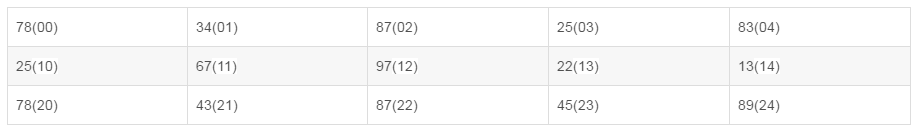
假设我有一张学生成绩表,成绩是按座位排列的,成绩表如下:

那么这张表的横轴就是排,竖轴就是列,我们可以算那一排或者那一列的平均分或者最高分,就是指定轴做运算,我们给张表当做一个二维数组并加上数组下标,变成下表:[78,34,87,25,83],[25,67,97,22,13],[78,43,87,45,89]]
运行代码求最大值:
import numpy as np

a = np.array([[78, 34, 87, 25, 83], [25, 67, 97, 22, 13], [78, 43, 87, 45, 89]])
print(a.max(axis=0))
print(a.max(axis=1))
'''
[78 67 97 45 89]
[87 97 89]
'''
从这里我们可以看到 axis=1 就是竖轴的数据,第一行打印了每列的最大值,axis=1就是横轴的数据。
下面我们再看一个2*2的三维数组:[[[0, 1], [2, 3]], [[4, 5], [6, 7]]]

运行代码求最大值:
import numpy as np

a = np.array([[[0, 1], [2, 3]], [[4, 5], [6, 7]]])
print(a)
print('**************************')
print(a.max(axis=0))
print('*************************')
print(a.max(axis=1))
print('**************************')
print(a.max(axis=2))
'''
[[[0 1]
  [2 3]]
 [[4 5]
  [6 7]]]
**************************
[[4 5]
 [6 7]]
*************************
[[2 3]
 [6 7]]
**************************
[[1 3]
 [5 7]]
'''
这里最大值就是把一个一维数组当成了一个元素,当axis为0和1时,和二维数组同理。
重点关注 axis=2时,这时为了匹配数组第三个下标相同的为一组,一维数组中的内容发生了改变:
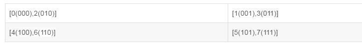
可以看出多维数组的axis是与数组下标相关的,现在可以学习rollaxis 函数了,这个函数有三个参数:
numpy.rollaxis(arr, axis, start)

arr:输入数组
axis:要向后滚动的轴,其它轴的相对位置不会改变
start:默认为零,表示完整的滚动。会滚动到特定位置
代码如下:
import numpy as np

a = np.arange(8).reshape(2, 2, 2)

print('原数组:')
print(a)
print('\n')
# 将轴 2 滚动到轴 0(宽度到深度)

print('调用 rollaxis 函数:')
print(np.rollaxis(a, 2))
# 将轴 0 滚动到轴 1:(宽度到高度)
print('\n')

print('调用 rollaxis 函数:')
print(np.rollaxis(a, 2, 1))
'''
原数组:
[[[0 1]
  [2 3]]
 [[4 5]
  [6 7]]]
调用 rollaxis 函数:
[[[0 2]
  [4 6]]
 [[1 3]
  [5 7]]]
调用 rollaxis 函数:
[[[0 2]
  [1 3]]
'''
程序运行 np.rollaxis(a, 2)时,将轴2滚动到了轴0前面,其他轴相对2轴位置不变(start默认0),数组下标排序由0, 1, 2 变成了 1, 2,0
这时候数组按下标顺序重组,例如第一个数组中 [0, 1] 下标为 [000, 001],其中0的下标变动不影响值,1位置的下标由001变成010,第一位的下标滚动到最后一位下标滚动到最后一位下标的后面,值由1(001)变成2(010):
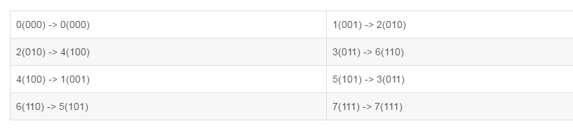
可以得出轴的滚动就是下标的滚动,同理,运行np.rollaxis(a, 2, 1)时将下标0,1,2变为0,2。
numpy.swapaxes(arr, axis1, axis2)函数则是交换,将axis1和axis2进行互换。
17,np.where() 函数
函数如下:
where(condition, x=None, y=None)
返回元素,可以是 x 或 y。具体取决于条件(condition),简单说就是满足条件,输出x,不满足输出y
如果只给出条件,则返回 condition.nonzero()
对于不同的输入,where返回的值是不同的。我们看例子
>>> aa = np.arange(10)
>>> np.where(aa,1,-1)
array([-1,  1,  1,  1,  1,  1,  1,  1,  1,  1])  # 0为False,所以第一个输出-1
>>> np.where(aa > 5,1,-1)
array([-1, -1, -1, -1, -1, -1,  1,  1,  1,  1])

>>> np.where([[True,False], [True,True]],    # 官网上的例子
			 [[1,2], [3,4]],
             [[9,8], [7,6]])
array([[1, 8],
	   [3, 4]])
上面这个例子的条件为 [ [True, False], [True, False]],分别对应最后输出结果的四个值,第一个值从 [1, 9]中选,因为条件是True,所以是选1,第二个值从 [2, 8] 中选,因为条件为False,所以选择8,后面依次类推,类似的问题可以再看个例子:
>>> a = 10
>>> np.where([[a > 5,a < 5], [a == 10,a == 7]],
             [["chosen","not chosen"], ["chosen","not chosen"]],
             [["not chosen","chosen"], ["not chosen","chosen"]])

array([['chosen', 'chosen'],
       ['chosen', 'chosen']], dtype='<U10')
只有条件(condition),没有x和y,则输出满足条件(即非0)元素的坐标(等价于 numpy.nonzero)。这里的坐标以 tuple 的形式给出,通常原数组有多少维,输出的 tuple中就包含几个数组,分别对应符合条件元素的各维坐标。
>>> a = np.array([2,4,6,8,10])
>>> np.where(a > 5)				# 返回索引
(array([2, 3, 4]),)
>>> a[np.where(a > 5)]  			# 等价于 a[a>5]
array([ 6,  8, 10])

>>> np.where([[0, 1], [1, 0]])
(array([0, 1]), array([1, 0]))
上面这个例子条件中 [[0, 1], [1, 0]] 的真值为两个 1,各自的第一维坐标为 [0, 1],第二维坐标 [1, 0]。
下面再看一个复杂的例子:
>>> a = np.arange(27).reshape(3,3,3)
>>> a
array([[[ 0,  1,  2],
        [ 3,  4,  5],
        [ 6,  7,  8]],

       [[ 9, 10, 11],
        [12, 13, 14],
        [15, 16, 17]],

       [[18, 19, 20],
        [21, 22, 23],
        [24, 25, 26]]])

>>> np.where(a > 5)
(array([0, 0, 0, 1, 1, 1, 1, 1, 1, 1, 1, 1, 2, 2, 2, 2, 2, 2, 2, 2, 2]),
 array([2, 2, 2, 0, 0, 0, 1, 1, 1, 2, 2, 2, 0, 0, 0, 1, 1, 1, 2, 2, 2]),
 array([0, 1, 2, 0, 1, 2, 0, 1, 2, 0, 1, 2, 0, 1, 2, 0, 1, 2, 0, 1, 2]))


# 符合条件的元素为
	   [ 6,  7,  8]],

      [[ 9, 10, 11],
       [12, 13, 14],
       [15, 16, 17]],

      [[18, 19, 20],
       [21, 22, 23],
       [24, 25, 26]]]
所以 np.where 会输出每个元素的对应的坐标,因为原数组有三维,所以 tuple中有三个数组。
18,np.diff() 函数
np.diff() 函数 是数组中 a[n] - a[n-1] 的结果
import numpy as np

a = np.array([1, 3, 5, 7, 9])
diff_a = np.diff(a)
print(diff_a)
# [2 2 2 2]
这个函数也适用于高维数组。
19,np.empty() 函数
np.empty()函数返回一个随机元素的矩阵,大小按照参数定义。所以使用的时候要小心,需要手工把每一个值重新定义,否则该值是一个随机数,调试起来比较麻烦。
def empty(shape, dtype=None, order='C'): # real signature unknown; restored from __doc__
    """
    empty(shape, dtype=float, order='C')

        Return a new array of given shape and type, without initializing entries.

        Parameters
        ----------
        shape : int or tuple of int
            Shape of the empty array, e.g., ``(2, 3)`` or ``2``.
        dtype : data-type, optional
            Desired output data-type for the array, e.g, `numpy.int8`. Default is
            `numpy.float64`.
        order : {'C', 'F'}, optional, default: 'C'
            Whether to store multi-dimensional data in row-major
            (C-style) or column-major (Fortran-style) order in
            memory.

        Returns
        -------
        out : ndarray
            Array of uninitialized (arbitrary) data of the given shape, dtype, and
            order.  Object arrays will be initialized to None.

        See Also
        --------
        empty_like : Return an empty array with shape and type of input.
        ones : Return a new array setting values to one.
        zeros : Return a new array setting values to zero.
        full : Return a new array of given shape filled with value.


        Notes
        -----
        `empty`, unlike `zeros`, does not set the array values to zero,
        and may therefore be marginally faster.  On the other hand, it requires
        the user to manually set all the values in the array, and should be
        used with caution.

        Examples
        --------
        >>> np.empty([2, 2])
        array([[ -9.74499359e+001,   6.69583040e-309],
               [  2.13182611e-314,   3.06959433e-309]])         #random

        >>> np.empty([2, 2], dtype=int)
        array([[-1073741821, -1067949133],
               [  496041986,    19249760]])                     #random
    """
官网有例子,我们这里稍微翻译下,他是依据给定形状和数据类型(order可以不用看)。(shape, [dtype, order]) 返回一个新的数组(可为空也可为其他,这是要给定的数据类型)。数据类型默认为 np.float64,索引当我们没有指定任何数据类型的时候,返回 i的数据肯定是 np.float64,即这时不可能为空。但是当数据类型是指对象的时候(比如list),会创建空数组。
a = np.empty((1, 4), dtype=dict)
print(a)  # [[None None None None]]
b = np.empty((1, 4), dtype=list)
print(b)  # [[None None None None]]
20,np.transpose()
(参考地址:https://www.freesion.com/article/149821286/)
首先看看源码:
    """
    Reverse or permute the axes of an array; returns the modified array.

    For an array a with two axes, transpose(a) gives the matrix transpose.

    Parameters
    ----------
    a : array_like
        Input array.
    axes : tuple or list of ints, optional
        If specified, it must be a tuple or list which contains a permutation of
        [0,1,..,N-1] where N is the number of axes of a.  The i'th axis of the
        returned array will correspond to the axis numbered ``axes[i]`` of the
        input.  If not specified, defaults to ``range(a.ndim)[::-1]``, which
        reverses the order of the axes.

    Returns
    -------
    p : ndarray
        `a` with its axes permuted.  A view is returned whenever
        possible.
    See Also
    --------
    moveaxis
    argsort

    Notes
    -----
    Use `transpose(a, argsort(axes))` to invert the transposition of tensors
    when using the `axes` keyword argument.

    Transposing a 1-D array returns an unchanged view of the original array.
参数 a:输入数组
axis:int 类型的列表,这个参数是可选的。默认情况下,反转的输入数组的维度,当给定这个参数时,按照这个参数所给定的值进行数组变换
返回值 p:ndarray 返回转置过后的原数组的视图
20.1 一维数组
对于1维数组,np.transpose() 是不起作用的,上面源码笔记也讲了,这里实验一下。
import numpy as np

t = np.arange(4)
# array([0, 1, 2, 3])
t.transpose()
# array([0, 1, 2, 3])
20.2 二维数组
二维数组的话,原数组有两个轴(x, y),对应的下标为(0, 1),np.transpose() 传入的参数为(1, 0),即将原数组的 x, y轴互换。所以对于二维数组的 transpose 操作就是对原数组的转置操作,实验如下:
import numpy as np

two_array = np.arange(16).reshape(4, 4)
# print(two_array)
'''
[[ 0  1  2  3]
 [ 4  5  6  7]
 [ 8  9 10 11]
 [12 13 14 15]]
'''
print(two_array.transpose())
'''
[[ 0  4  8 12]
 [ 1  5  9 13]
 [ 2  6 10 14]
 [ 3  7 11 15]]
'''
print(two_array.transpose(1, 0))
'''
[[ 0  4  8 12]
 [ 1  5  9 13]
 [ 2  6 10 14]
 [ 3  7 11 15]]
'''
20.3 三维数组
对于三维数组,我们可以先看一个例子:
import numpy as np

three_array = np.arange(18).reshape(2, 3, 3)
# print(three_array)
'''
[[[ 0  1  2]
  [ 3  4  5]
  [ 6  7  8]]
 [[ 9 10 11]
  [12 13 14]
  [15 16 17]]]
'''
print(three_array.transpose())
'''
[[[ 0  9]
  [ 3 12]
  [ 6 15]]
 [[ 1 10]
  [ 4 13]
  [ 7 16]]
 [[ 2 11]
  [ 5 14]
  [ 8 17]]]
'''
这是 np.transpose()函数对 three_array 数组默认的操作,即将原数组的各个 axis 进行 reverse一下,three_array的原始 axis 排列为(0, 1, 2),numpy.transpose() 默认的参数为(2, 1, 0)得到转置后的数组的视图,不影响原数组的内容以及大小。我们一步一步来分析这个过程:axis(0, 1, 2)——> axis(2, 1, 0),transpose后的数组对于原数组来说,相当于交换了原数组的 0轴和 2轴。
#对原始three数组的下标写出来,如下:
A=[
       [ [ (0,0,0) , (0,0,1) , (0,0,2)],
       [ (0,1,0) , (0,1,1) , (0,1,2)],
       [ (0,2,0) , (0,2,1) , (0,2,2)]],

       [[ (1,0,0) , (1,0,1) , (1,0,2)],
        [ (1,1,0) , (1,1,1) , (1,1,2)],
        [ (1,2,0) , (1,2,1) , (1,2,2)]]
  ]

#接着把上述每个三元组的第一个数和第三个数进行交换,得到以下的数组

B=[[[ (0,0,0) , (1,0,0) , (2,0,0)],
  [ (0,1,0) , (1,1,0) , (2,1,0)],
  [ (0,2,0) , (1,2,0) , (2,2,0)]],

  [[ (0,0,1) , (1,0,1) , (2,0,1)],
  [ (0,1,1) , (1,1,1) , (2,1,1)],
  [ (0,2,1) , (1,2,1) , (2,2,1)]]]

#最后在原数组中把B对应的下标的元素,写到相应的位置
#对比看一下,这是原数组
[[[ 0,  1,  2],
  [ 3,  4,  5],
  [ 6,  7,  8]],

  [[ 9, 10, 11],
   [12, 13, 14],
   [15, 16, 17]]]
# 按照B的映射关系得到最终的数组。
C=[[[ 0,  9],
  [ 3,  12],
  [ 6,  15]],

  [[ 1, 10],
   [4, 13],
   [7, 16]]

   [[ 2, 11],
   [5, 14],
   [8, 17]]
]
# 最终的结果也就是数组C
我们知道旋转的矩阵结果,那么在深度学习中为什么要这么旋转图片呢?以及这样做的意义是什么呢?我们可以继续学习:
import cv2 as cv
import numpy as np


img = cv.imread('my.jpg')
cv.imshow('img',img)
#逆时针旋转90度
img = np.transpose(img, (1, 0, 2))
#顺时针旋转90度
# img = cv.flip(img, 1)
#顺时针旋转270度
# img = cv.flip(img, 1)
cv.namedWindow('img',cv.WINDOW_AUTOSIZE)
cv.imshow('img2',img)
cv.waitKey(0)
cv.destroyAllWindows()
对图像执行 np.transpse(img, (1, 0, 2)) 操作,可以将图像逆时针翻转 90度,在配合 cv2.fip(img, 0 or 1),可以做到翻转 270度或 90度。
下面函数也是翻转图像的,可以继续看一下,自己喜欢那个用那个。
21,np.rot90()
此函数的功能是旋转矩阵(矩阵逆时针旋转90度或者90度的倍数),有时可以用来旋转图像。
函数源码如下(m为待旋转的矩阵,k为旋转角度为90度*K(k默认为1)):
def rot90(m, k=1, axes=(0, 1)):
    """
    Rotate an array by 90 degrees in the plane specified by axes.

    Rotation direction is from the first towards the second axis.

    Parameters
    ----------
    m : array_like
        Array of two or more dimensions.
    k : integer
        Number of times the array is rotated by 90 degrees.
    axes: (2,) array_like
        The array is rotated in the plane defined by the axes.
        Axes must be different.

        .. versionadded:: 1.12.0

    Returns
    -------
    y : ndarray
        A rotated view of `m`.

    See Also
    --------
    flip : Reverse the order of elements in an array along the given axis.
    fliplr : Flip an array horizontally.
    flipud : Flip an array vertically.

    Notes
    -----
    rot90(m, k=1, axes=(1,0)) is the reverse of rot90(m, k=1, axes=(0,1))
    rot90(m, k=1, axes=(1,0)) is equivalent to rot90(m, k=-1, axes=(0,1))
示例:
    >>> m = np.array([[1,2],[3,4]], int)
    >>> m
    array([[1, 2],
           [3, 4]])
    >>> np.rot90(m)
    array([[2, 4],
           [1, 3]])
    >>> np.rot90(m, 2)
    array([[4, 3],
           [2, 1]])
    >>> m = np.arange(8).reshape((2,2,2))
    >>> np.rot90(m, 1, (1,2))
    array([[[1, 3],
            [0, 2]],
           [[5, 7],
            [4, 6]]])
还有两种旋转图像的方法,是使用PIL,但是会改变图像尺寸。需要注意使用。旋转包括 transpose() 和 rotate() 两种方式。
from PIL import Image

img = Image.open("logo1.jpg")

# 旋转方式一
img1 = img.transpose(Image.ROTATE_90)   # 引用固定的常量值
img1.save("r1.jpg")

# 旋转方式二
img2 = img.rotate(90)   # 自定义旋转度数
img2.save("r2.jpg")

# np  旋转方式
img3 = cv2.imread("logo1.jpg")
img3 = np.rot90(img3, k=1)
cv2.imwrite("r3.jpg", img3)
我们看看效果:

所以,慎重使用rotate,我就踩坑了。
参考文献:https://github.com/wmpscc/DataMiningNotesAndPractice/blob/master/4.NumPy%E5%AD%A6%E4%B9%A0%E7%AC%94%E8%AE%B0.md

 浙公网安备 33010602011771号