Tensorflow2.0笔记14——常用Tensorflow API及代码实现

Tensorflow2.0笔记

本博客为Tensorflow2.0学习笔记，感谢北京大学微电子学院曹建老师

目录

• Tensorflow2.0笔记
  • 7.常用Tensorflow API及代码实现
    • 7.1学习率策略
      • tf.keras.optimizers.schedules.ExponentialDecay
      • tf.keras.optimizers.schedules.PiecewiseConstantDecay
    • 7.2激活函数
      • tf.math.sigmoid
      • tf.math.tanh
      • tf.nn.relu
      • tf.nn.softmax

7.常用Tensorflow API及代码实现

7.1学习率策略

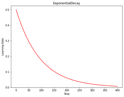
tf.keras.optimizers.schedules.ExponentialDecay

tf.keras.optimizers.schedules.ExponentialDecay(
	initial_learning_rate, decay_steps, decay_rate, staircase=False, name=None
)

功能：指数衰减学习率策略.

等价API：tf.optimizers.schedules.ExponentialDecay

参数：

​ initial_learning_rate: 初始学习率

​ decay_steps: 衰减步数, staircase为True时有效.

​ decay_rate: 衰减率

​ staircase: Bool型变量.如果为True, 学习率呈现阶梯型下降趋势.

返回：tf.keras.optimizers.schedules.ExponentialDecay(step)返回计算得到的学习率

链接：tf.keras.optimizers.schedules.ExponentialDecay

示例：

N = 400
lr_schedule = 
	tf.keras.optimizers.schedules.ExponentialDecay( 0.5,
	decay_steps=10, 
	decay_rate=0.9, 
	staircase=False)
y = []
for global_step in range(N):
	lr = lr_schedule(global_step) 
	y.append(lr)
x = range(N) 
plt.figure(figsize=(8,6)) 
plt.plot(x, y, 'r-')
plt.ylim([0,max(plt.ylim())]) 
plt.xlabel('Step') 
plt.ylabel('Learning Rate') 
plt.title('ExponentialDecay') 
plt.show()

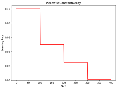
tf.keras.optimizers.schedules.PiecewiseConstantDecay

tf.keras.optimizers.schedules.PiecewiseConstantDecay( 
	boundaries, values, name=None
)

功能：分段常数衰减学习率策略.

等价API：tf.optimizers.schedules.PiecewiseConstantDecay

参数：

​ boundaries: [step_1, step_2, ..., step_n]定义了在第几步进行学习率衰减

​ values: [val_0, val_1, val_2, ..., val_n]定义了学习率的初始值和后续衰减时的具体取值

返回：tf.keras.optimizers.schedules.PiecewiseConstantDecay(step)返回计算得到的学习率.

链接： tf.keras.optimizers.schedules.PiecewiseConstantDecay

示例：

N = 400
lr_schedule = 
	tf.keras.optimizers.schedules.PiecewiseConstantDecay( 
	boundaries=[100, 200, 300],
	values=[0.1, 0.05, 0.025, 0.001]) 
y = []
for global_step in range(N):
	lr = lr_schedule(global_step) 
	y.append(lr)
x = range(N) 
plt.figure(figsize=(8,6)) 
plt.plot(x, y, 'r-')
plt.ylim([0,max(plt.ylim())]) 
plt.xlabel('Step') 
plt.ylabel('Learning Rate') 
plt.title('PiecewiseConstantDecay')

7.2激活函数

tf.math.sigmoid

tf.math.sigmoid( 
	x, name=None
)

功能：计算x每一个元素的sigmoid值.

等价API：tf.nn.sigmoid, tf.sigmoid

参数：

​ x是张量x

返回：

​ 与x shape相同的张量

链接： tf.math.sigmoid

示例：

x = tf.constant([1., 2., 3.], ) 
print(tf.math.sigmoid(x))

>>> tf.Tensor([0.7310586 0.880797  0.95257413], shape=(3,), dtype=float32)

# 等价实现
print(1/(1+tf.math.exp(-x)))

>>> tf.Tensor([0.7310586  0.880797  0.95257413], shape=(3,), dtype=float32)

tf.math.tanh

tf.math.tanh(
	x, name=None
)

功能：计算x每一个元素的双曲正切值.

等价API：tf.nn.tanh, tf.tanh

参数：

​ x是张量x

返回：

​ 与x shape相同的张量

链接： tf.math.tanh

示例：

x = tf.constant([-float("inf"), -5, -0.5, 1, 1.2, 2, 3, float("inf")]) 
print(tf.math.tanh(x))

>>> tf.Tensor([-1. -0.99990916 -0.46211717 0.7615942 0.8336547 0.9640276
0.9950547 1.], shape=(8,), dtype=float32)

# 等价实现
print((tf.math.exp(x)-tf.math.exp(-x))/(tf.math.exp(x)+tf.math.exp(-x)))

>>> tf.Tensor([nan -0.9999091 -0.46211714 0.7615942 0.83365464 0.9640275
0.9950547 nan], shape=(8,), dtype=float32)

tf.nn.relu

tf.nn.relu(
	features, name=None
)

功能：计算修正线性值(rectified linear)：max(features, 0).

参数：

​ features：张量

链接： tf.nn.relu

例子：

print(tf.nn.relu([-2., 0., -0., 3.]))

>>> tf.Tensor([0. 0. -0. 3.], shape=(4,), dtype=float32)

tf.nn.softmax

tf.nn.softmax(
	logits, axis=None, name=None
)

功能：计算softmax激活值.

等价API：tf.math.softmax

参数：

​ logits：张量

​ axis：计算softmax所在的维度. 默认为-1，即最后一个维度

返回：与logits shape相同的张量.

链接： tf.nn.softmax

logits = tf.constant([4., 5., 1.]) 
print(tf.nn.softmax(logits))

>>> tf.Tensor([0.26538792 0.7213992 0.01321289], shape=(3,), dtype=float32)

# 等价实现
print(tf.exp(logits) / tf.reduce_sum(tf.exp(logits)))

\>>> tf.Tensor([0.26538792 0.72139925 0.01321289], shape=(3,), dtype=float32)