


ISLR第8章The Basics of Decision Trees
The Basics of Decision Trees
In this chapter, we describe tree-based methods for regression and classification.
These involve stratifying or segmenting the predictor space into a number of simple regions.
In order to make a prediction for a given observation, we typically use the mean or the mode
of the training observations in the region to which it belongs. Since the set of splitting rules
used to segment the predictor space can be summarized in a tree, these types of approaches
are known as decision tree methods.
Tree-based methods are simple and useful for interpretation. However, they typically are not
competitive with the best supervised learning approaches, such as those seen in Chapters 6 and 7,
in terms of prediction accuracy. Hence in this chapter we also introduce bagging, random forests,
and boosting. Each of these approaches involves producing multiple trees which are then combined
to yield a single consensus prediction. We will see that combining a large number of trees can often
result in dramatic improvements in prediction accuracy, at the expense of some loss in interpretation.
8.1 The Basics of Decision Trees
Decision trees can be applied to both regression and classification problems.
We first consider regression problems, and then move on to classification

8.1.1Regression Trees
Prediction via Stratification of the Feature Space
We now discuss the process of building a regression tree. Roughly speaking, there are two steps.
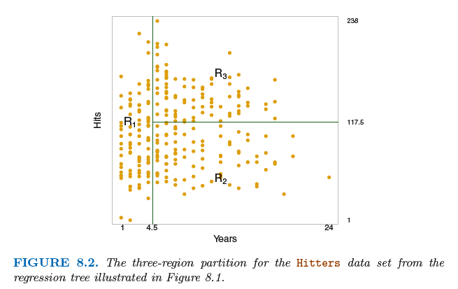
1. We divide the predictor space—that is, the set of possible values for X1,X2, . . .,Xp—into J distinct(不同的) and non-overlapping(非重叠的)
regions,R1,R2, . . . , RJ .
2. For every observation that falls into the region Rj, we make the same prediction, which is simply the mean of the response values for the
training observations in Rj .
We now elaborate on Step 1 above. How do we construct the regions R1, . . .,RJ? In theory, the regions could have any shape.
However, we choose to divide the predictor space into high-dimensional rectangles, or boxes, for simplicity and for ease of
interpretation of the resulting predictive model. The goal is to find boxes R1, . . . , RJ that minimize the RSS, given by
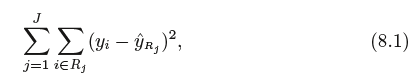
where ˆyRj is the mean response for the training observations within the jth box. Unfortunately, it is computationally infeasible to
consider every possible partition of the feature space into J boxes. For this reason, we take a top-down, greedy approach that
is known as recursive binary splitting(递归二分裂)
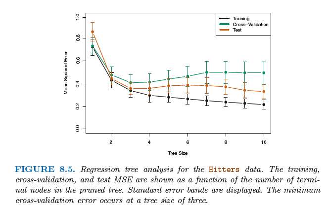
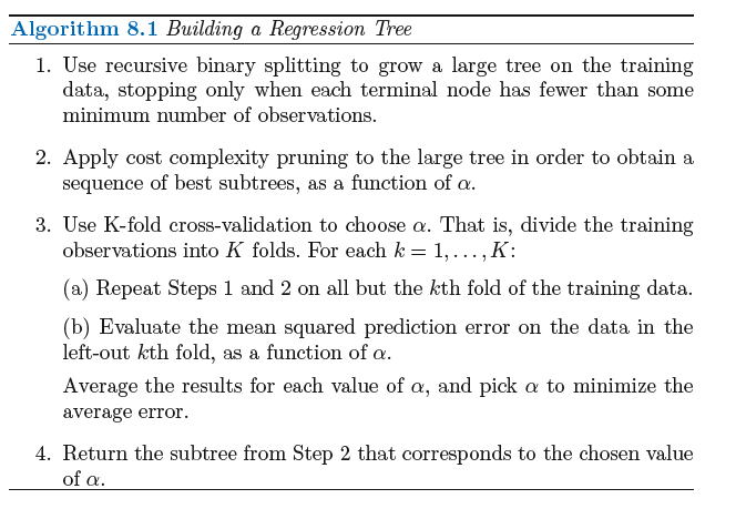
Tree Pruning(树修剪)
The process described above may produce good predictions on the training set, but is likely to overfit the data, leading to poor test
set performance. This is because the resulting tree might be too complex .Therefore, a better strategy is to grow a very large tree T0,
and then prune it back in order to obtain a subtree.
Cost complexity pruning—also known as weakest link pruning—gives us a way to do just this. Rather than considering every possible
subtree, we consider a sequence of trees indexed by a nonnegative tuning parameter α.
For each value of α there corresponds a subtree T ⊂ T0 such that
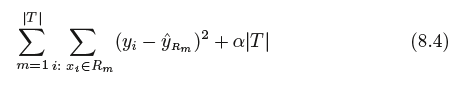
is as small as possible.
Here |T | indicates the number of terminal nodes of the tree T , Rm is the rectangle (i.e. the subset of predictor space) corresponding
to the mth terminal node, and ˆyRm is the predicted response associated with Rm—that is, the mean of the training observations in Rm.
The tuning parameter α controls a trade-off between the subtree’s complexity and its fit to the training data. When α = 0, then the subtree T
will simply equal T0, because then (8.4) just measures the training error. However, as α increases, there is a price to pay for having a tree with
many terminal nodes, and so the quantity (8.4) will tend to be minimized for a smaller subtree.
8.1.2 Classification Trees
The task of growing a classification tree is quite similar to the task of growing a regression tree. Just as in the regression setting,
we use recursive binary splitting to grow a classification tree. However, in the classification setting, RSS cannot be used as a
criterion for making the binary splits. A natural alternative to RSS is the classification error rate. Since we plan classification
to assign an observation in a given region to the most commonly occurring error rate class of training observations in that region,
the classification error rate is simply the fraction of the training observations in that region that do not belong to the most common class:
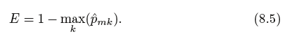
Here ˆpmk represents the proportion of training observations in the mth region that are from the kth class. However, it turns out that classification
error is not sufficiently sensitive for tree-growing, and in practice two other measures are preferable.
The Gini index(基尼系数) is defined by
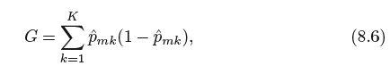
a measure of total variance across the K classes. It is not hard to see that the Gini index takes on a small value if all of the ˆpmk’s are close to
zero or one. For this reason the Gini index is referred to as a measure of node purity—a small value indicates that a node contains predominantly
observations from a single class.(一个小的基尼系数表示一个节点包含的观测主要来自一个单的分类).
An alternative to the Gini index is entropy, given by
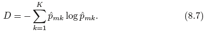
Therefore, like the Gini index, the entropy will take on a small value if the mth node is pure. In fact, it turns out that the Gini nindex and the entropy
are quite similar numerically.
8.1.3 Trees Versus Linear Models
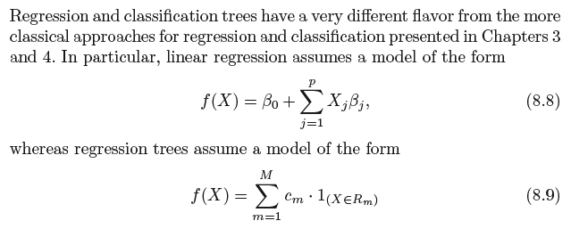
where R1, . . .,RM represent a partition of feature space
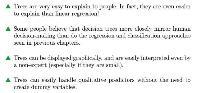
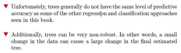
8.1.4 Advantages and Disadvantages of Trees
8.2 Bagging, Random Forests, Boosting
8.2.1 Bagging
In other words, averaging a set of observations reduces variance. Hence a natural way to reduce the variance and hence increase the prediction accuracy of a statistical learning
method is to take many training sets from the population, build a separate prediction model using each training set, and average the resulting predictions.
Instead, we can bootstrap, by taking repeated samples from the (single) training data set. In this approach we generate B different bootstrapped training data sets. We then train our method on the bth bootstrapped training set in order to get ˆ f∗b(x), and finally average all the predictions, to obtain
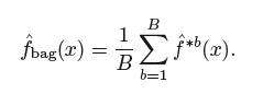
This is called bagging.
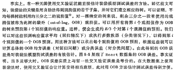
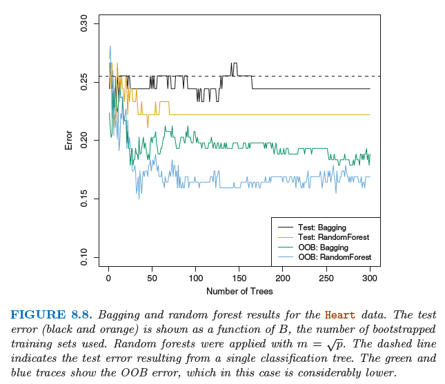
Out-of-Bag Error Estimation(袋外误差估计)
It turns out that there is a very straightforward way to estimate the test error of a bagged model, without the need to perform cross-validation or the validation set approach.
Recall that the key to bagging is that trees are repeatedly fit to bootstrapped subsets of the observations. One can show that on average, each bagged tree makes use of around two-thirds of the observations.3 The remaining one-third of the observations not used to fit a given bagged tree are referred to as the out-of-bag (OOB) observations.
8.2.2 Random Forests随机森林
随机森林是对袋装法树的改进。在随机森林中需要对自助抽样训练集建立一系列的决策树,这与袋装树类似。
不过在建立这些决策树时,每考虑树上的一个分裂点,都要从全部的p个预测变量中选出一个包含m个预测变量
的随机样本作为候选变量。这个分裂点所用的预测变量只能从这个m个变量中选择。在每个分裂点处都需要进行
重新抽样,选出m个预测变量,通常m=根号下p。
袋装法和随机森林最大的不同在于预测变量子集的规模m。当m=p时,建立的随机森林等同与袋装树。
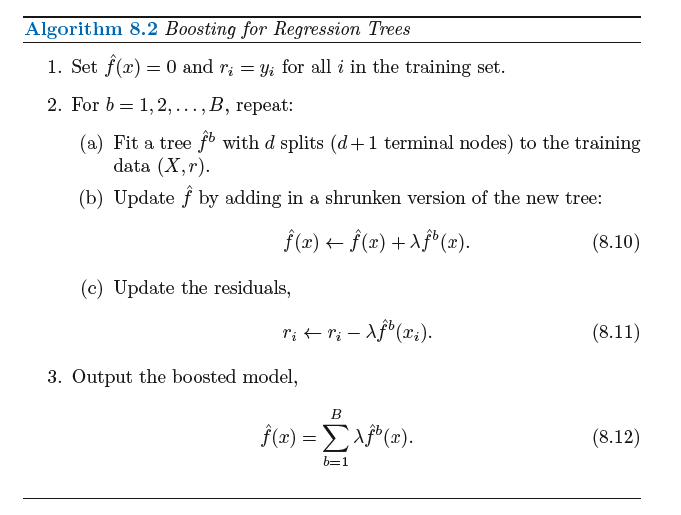
8.2.3 Boosting提升法
提升法的树都是顺序生成的,每棵树的建立都需要用到之前生成的树中的信息。
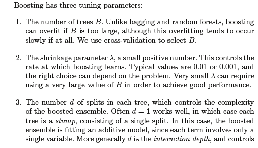
提升法的三个调节参数:

 浙公网安备 33010602011771号