第八章习题

学号后四位:3018
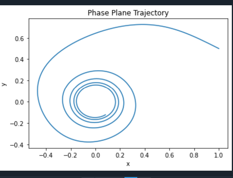
8.4:

点击查看代码

import numpy as np
from scipy.integrate import odeint
import matplotlib.pyplot as plt


# 定义微分方程组
def differential_equations(state, t):
    x, y = state
    dxdt = -x ** 3 - y
    dydt = x - y ** 3
    return [dxdt, dydt]


# 设定初始条件
initial_conditions = [1, 0.5]

# 定义时间范围
t = np.linspace(0, 30, 1000)

# 求解微分方程组
solution = odeint(differential_equations, initial_conditions, t)
x_solution = solution[:, 0]
y_solution = solution[:, 1]

# 绘制x(t)的解曲线
plt.subplot(2, 1, 1)
plt.plot(t, x_solution)
plt.xlabel('t')
plt.ylabel('x(t)')
plt.title('Solution Curve of x(t)')

# 绘制y(t)的解曲线
plt.subplot(2, 1, 2)
plt.plot(t, y_solution)
plt.xlabel('t')
plt.ylabel('y(t)')
plt.title('Solution Curve of y(t)')

# 在相平面上绘制轨线
plt.figure()
plt.plot(x_solution, y_solution)
plt.xlabel('x')
plt.ylabel('y')
plt.title('Phase Plane Trajectory')

plt.show()
print("xuehao3018")

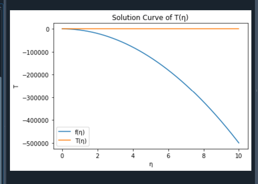
8.5:

点击查看代码

import numpy as np
from scipy.integrate import odeint
import matplotlib.pyplot as plt

# 定义微分方程组
def equations(state, eta):
    f, df_deta, T, dT_deta = state
    # 用中心差分近似计算二阶导数
    h = 1e-4
    df2_deta2_approx = (state[1] - odeint(equations, [state[0]+h, df_deta+h, state[2], dT_deta], [eta])[0][1]) / h**2
    d2T_deta2 = -2.1 * f * dT_deta
    return [df_deta, df2_deta2_approx, dT_deta, d2T_deta2]

# 初始条件
f0 = 0
df_deta0 = -0.5
T0 = 1
dT_deta0 = 0
initial_conditions = [f0, df_deta0, T0, dT_deta0]

# 定义 eta 的范围
eta = np.linspace(0, 10, 1000)

# 求解微分方程组
solution = odeint(equations, initial_conditions, eta)
f_solution = solution[:, 0]
T_solution = solution[:, 2]

# 绘制 f(η) 的解曲线
plt.plot(eta, f_solution, label='f(η)')
plt.xlabel('η')
plt.ylabel('f')
plt.title('Solution Curve of f(η)')

# 绘制 T(η) 的解曲线
plt.plot(eta, T_solution, label='T(η)')
plt.xlabel('η')
plt.ylabel('T')
plt.title('Solution Curve of T(η)')

plt.legend()
plt.show()
print("xuehao3018")

8.7:

点击查看代码

import numpy as np
import matplotlib.pyplot as plt
from scipy.integrate import odeint

def pendulum_ode_1(y, t, g, l):
    theta, omega = y
    dydt = [omega, -g / l * np.sin(theta)]
    return dydt

l = 1
g = 9.8
theta_0 = 15 / 180 * np.pi
y0 = [theta_0, 0]
t = np.linspace(0, 30, 1000)
sol_1 = odeint(pendulum_ode_1, y0, t, args=(g, l))

plt.plot(t, sol_1[:, 0])
plt.xlabel('t')
plt.ylabel('theta(t)')
plt.title('Pendulum without viscous medium')
plt.show()

def pendulum_ode_2(y, t, g, l, lambda_):
    theta, omega = y
    dydt = [omega, -g / l * np.sin(theta) - lambda_ / l * omega]
    return dydt

lambda_ = 0.1
y0 = [theta_0, 0]
sol_2 = odeint(pendulum_ode_2, y0, t, args=(g, l, lambda_))

plt.plot(t, sol_2[:, 0])
plt.xlabel('t')
plt.ylabel('theta(t)')
plt.title('Pendulum with viscous medium')
plt.show()
print("xuehao3018")

8.8:

点击查看代码

import numpy as np
from scipy.integrate import odeint
import matplotlib.pyplot as plt


# 定义参数
b3 = 0.5 * 1.109 * 10**5
b4 = 1.109 * 10**5
s = lambda n: 1.22 * 10**11 / (1.22 * 10**11 + n)
d = 0.8
w3 = 17.86
w4 = 22.99
q3 = 0.42
q4 = 1
E = 1  # 初始捕捞努力量，后面会进行优化


def fish_model(x, t):
    x1, x2, x3, x4 = x
    n = b3 * x3 + b4 * x4
    dx1dt = (b3 * x3 + b4 * x4) * s(n) - d * x1
    dx2dt = x1 * (1 - d) - d * x2
    dx3dt = x2 * (1 - d) - d * x3 - q3 * E * x3
    dx4dt = x3 * (1 - d) - d * x4 - q4 * E * x4
    return [dx1dt, dx2dt, dx3dt, dx4dt]


# 初始鱼群数量
x0 = [1000, 1000, 1000, 1000]
t = np.linspace(0, 10, 1000)
sol = odeint(fish_model, x0, t)


# 计算捕捞量
def calculate_yield(x, E):
    x3, x4 = x[2], x[3]
    return (w3 * q3 * E * x3 + w4 * q4 * E * x4)


# 寻找最优捕捞努力量（简单示例，实际可能需要更复杂的优化算法）
Es = np.linspace(0, 5, 100)
yields = []
for e in Es:
    E = e
    sol = odeint(fish_model, x0, t)
    x_end = sol[-1]
    yield_value = calculate_yield(x_end, E)
    yields.append(yield_value)

optimal_E_index = np.argmax(yields)
optimal_E = Es[optimal_E_index]


# 绘制结果
plt.plot(Es, yields)
plt.xlabel('Fishing Effort (E)')
plt.ylabel('Yield')
plt.title('Optimal Fishing Strategy')
plt.show()
print("xuehao3018")

8.9:

点击查看代码

import numpy as np

# 购房总价
total_price = 600000
# 首付
down_payment = 200000
# 贷款本金
loan_principal = total_price - down_payment
# 月利率
monthly_interest_rate = 0.0036
# 贷款期限（月数）
loan_months = 30 * 12

# 计算月还款额
monthly_payment = loan_principal * (monthly_interest_rate * (1 + monthly_interest_rate) ** loan_months) / ((1 + monthly_interest_rate) ** loan_months - 1)
print("月还款额为：", round(monthly_payment, 2))
print("xuehao3018")