数据挖掘实战：信用卡违约率分析

 

【项目目标】

这个数据集是台湾某银行 2005 年 4 月到 9 月的信用卡数据，数据集一共包括 25 个字段，现在我们的目标是要采用随机森林算法，针对这个数据集构建一个分析信用卡违约率的分类器。

【项目过程】

1.数据获取

2.数据探索、数据规范化、数据集划分

3.模型创建、模型训练、模型评估

【项目实现】

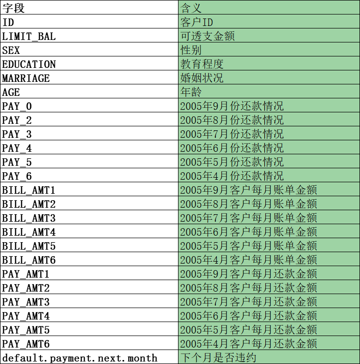
每个字段的含义如下：

 1.导库

import pandas as pd
from sklearn.model_selection import GridSearchCV
from sklearn.preprocessing import StandardScaler
from sklearn.ensemble import RandomForestClassifier
from matplotlib import pyplot as plt

2.导入数据、探索数据

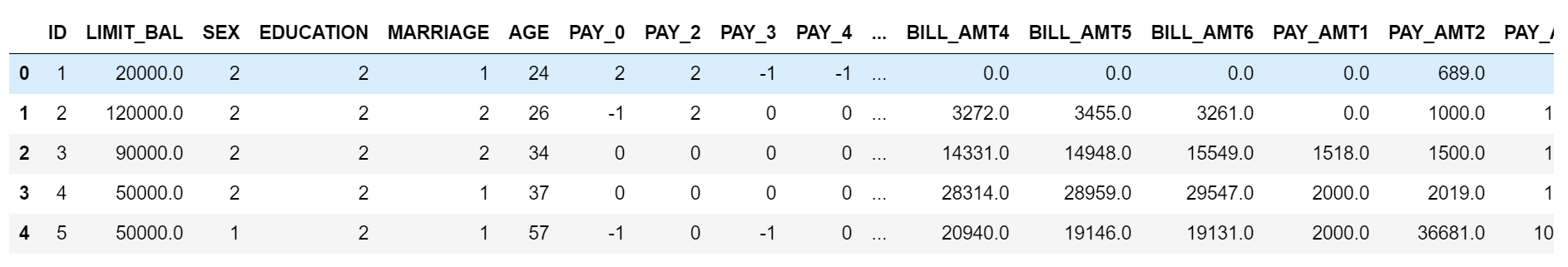
data = pd.read_csv("./UCI_Credit_Card.csv")
data.shape

(30000, 25)

data.head()

data.info()

<class 'pandas.core.frame.DataFrame'>
RangeIndex: 30000 entries, 0 to 29999
Data columns (total 25 columns):
 #   Column                      Non-Null Count  Dtype  
---  ------                      --------------  -----  
 0   ID                          30000 non-null  int64  
 1   LIMIT_BAL                   30000 non-null  float64
 2   SEX                         30000 non-null  int64  
 3   EDUCATION                   30000 non-null  int64  
 4   MARRIAGE                    30000 non-null  int64  
 5   AGE                         30000 non-null  int64  
 6   PAY_0                       30000 non-null  int64  
 7   PAY_2                       30000 non-null  int64  
 8   PAY_3                       30000 non-null  int64  
 9   PAY_4                       30000 non-null  int64  
 10  PAY_5                       30000 non-null  int64  
 11  PAY_6                       30000 non-null  int64  
 12  BILL_AMT1                   30000 non-null  float64
 13  BILL_AMT2                   30000 non-null  float64
 14  BILL_AMT3                   30000 non-null  float64
 15  BILL_AMT4                   30000 non-null  float64
 16  BILL_AMT5                   30000 non-null  float64
 17  BILL_AMT6                   30000 non-null  float64
 18  PAY_AMT1                    30000 non-null  float64
 19  PAY_AMT2                    30000 non-null  float64
 20  PAY_AMT3                    30000 non-null  float64
 21  PAY_AMT4                    30000 non-null  float64
 22  PAY_AMT5                    30000 non-null  float64
 23  PAY_AMT6                    30000 non-null  float64
 24  default.payment.next.month  30000 non-null  int64  
dtypes: float64(13), int64(12)
memory usage: 5.7 MB

通过data.info()发现数据很完整，没有缺失值，不需要进行缺失值的处理

分析数据特征的类型可以发现，数据分为分类型变量和数值型变量，其中 SEX/EDUCATION/MARRIAGE 为分类型变量，其中 SEX 为无序数据，应该采用 OneHotEncoder 编码

看一下标签的分类情况

data["default.payment.next.month"].value_counts()

0    23364
1     6636
Name: default.payment.next.month, dtype: int64

df = pd.DataFrame({'default.payment.next.month': next_month.index,'values': next_month.values})

plt.rcParams['font.sans-serif']=['SimHei'] # 用来正常显示中文标签
plt.figure()
plt.bar(["0","1"],df["values"],)
plt.title('信用卡违约率客户\n (违约：1，守约：0)')

 

可以看到，不存在严重的样本不均衡问题

接下来对 SEX 进行独热编码

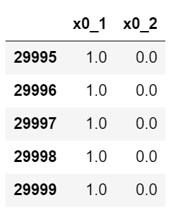
from sklearn.preprocessing import OneHotEncoder

ohe = OneHotEncoder(sparse=False)
ohe.fit(data["SEX"].values.reshape(-1, 1))
SEX_df = pd.DataFrame(ohe.transform(data["SEX"].values.reshape(-1, 1)), columns=ohe.get_feature_names())
SEX_df.tail()

 

 删除无用字段 SEX ID

data.drop(["SEX","ID"], inplace=True, axis=1)

# 分类型变量
data_cv = pd.concat([data.iloc[:,[1,2]],SEX_df],axis=1)
data_cv

# 数值型变量 
data_mv = pd.concat([data["LIMIT_BAL"],data.iloc[:,3:22]],axis=1)
data_mv

# 数值型变量归一化 
ss = StandardScaler()
data_mv_std = ss.fit_transform(data_mv)
data_mv_std_df = pd.DataFrame(data_mv_std)
data_mv_std_df

# 划分特征与标签
features = pd.concat([data_mv_std_df,data_cv],axis=1)
target = data.iloc[:,-1]

使用GridSearchCV对随机森林分类器进行超参数选择

rfc = RandomForestClassifier(n_jobs=-1,max_features= 'sqrt' ,n_estimators=50, oob_score = True) 

param_grid = { 
    'n_estimators': [50,200],
    'max_features': ['auto', 'sqrt', 'log2']
}

CV_rfc = GridSearchCV(estimator=rfc, param_grid=param_grid, cv= 5)
CV_rfc.fit(features, target)

CV_rfc.best_params_

{'max_features': 'log2', 'n_estimators': 200}

CV_rfc.best_score_

0.8164