轻松拿下91%准确率 | 利用PyTorch搞定Fashion-MNIST
作者:如缕清风
本文为博主原创,未经允许,请勿转载:https://www.cnblogs.com/warren2123/p/15035742.html
一、前言
本文通过PyTorch构建简单的卷积神经网络模型,实现对图像分类入门数据——Fashion-MNIST进行分类。
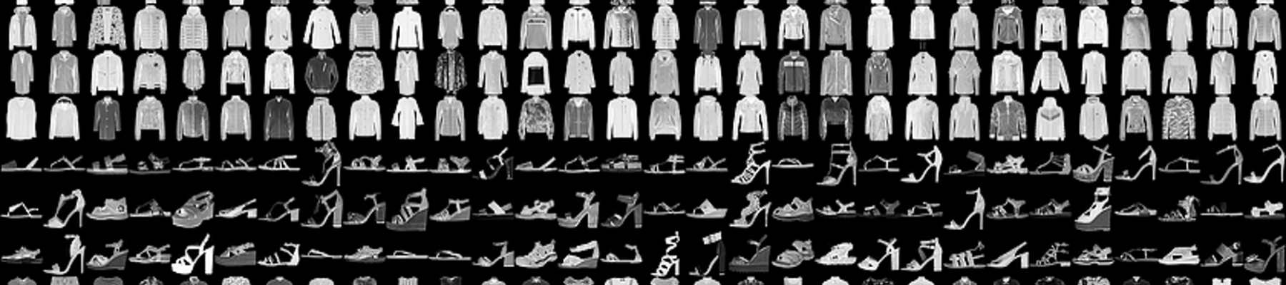
Fashion-MNIST 是 Zalando 文章图像的数据集,由 60,000 个示例的训练集和 10,000 个示例的测试集组成。每个示例都是一个 28x28 灰度图像,共分为 10 个类别。Fashion-MNIST样本图例如下所示:
二、基于PyTorch构建卷积神经网络模型
由于Fashion-MNIST数据比较简单,仅有一个通道的灰度图像,通过叠加几层卷积层并结合超参数优化,轻松实现91%以上的准确率。本文模型构建分为五个部分:数据读取及预处理、构建卷积神经网络模型、定义模型超参数以及评估方法、参数更新、优化。
1、数据读取及预处理
以下是本文用到的Python库,同样采用GPU进行运算加速,若不存在GPU,则会采用CPU进行运算。
import numpy as np
import pandas as pd
import torch
import torch.nn as nn
import torch.nn.functional as F
from torch.utils.data import Dataset, DataLoader
from pathlib import Path
device = torch.device("cuda:0" if torch.cuda.is_available() else "cpu")
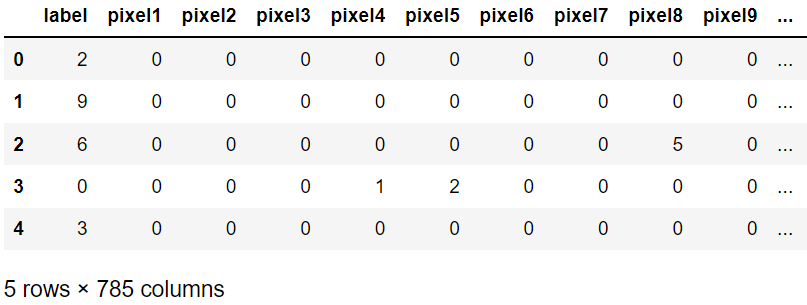
由于文件采用csv格式文件,所以采取Pandas对文件进行读取。数据有785列,其中label为标签值。
DATA_PATH = Path('data/')
train = pd.read_csv(DATA_PATH / "fashion-mnist_train.csv")
train.head()
通过继承PyTorch的Dataset方法,定义一个处理Fashion-MNIST的类。
class FashionMNISTDataset(Dataset):
    def __init__(self, csv_file, transform=None):
        data = pd.read_csv(csv_file)
        self.X = np.array(data.iloc[:, 1:]).reshape(-1, 1, 28, 28).astype(float)
        self.Y = np.array(data.iloc[:, 0])
        del data
        self.len = len(self.X)

    def __len__(self):
        return self.len

    def __getitem__(self, idx):
        item = self.X[idx]
        label = self.Y[idx]
        return (item, label)
首先运用定义的FashionMNISTDataset将数据集变换成 28x28 的格式,再用DataLoader的方法读取数据。
train_dataset = FashionMNISTDataset(csv_file=DATA_PATH / "fashion-mnist_train.csv")
test_dataset = FashionMNISTDataset(csv_file=DATA_PATH / "fashion-mnist_test.csv")

train_loader = DataLoader(dataset=train_dataset, batch_size=BATCH_SIZE, shuffle=True)
test_loader = DataLoader(dataset=test_dataset, batch_size=BATCH_SIZE, shuffle=False)
2、构建卷积神经网络模型
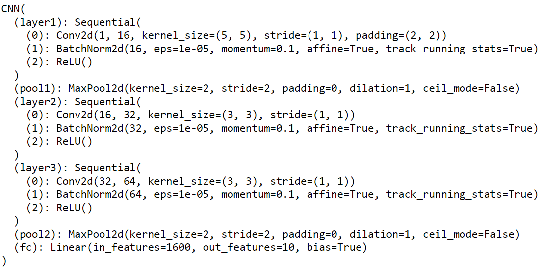
本文的卷积神经网络模型,采用三层卷积层、两层池化层、一层全连接层,卷积层都运用批量归一化的方法以便提升模型泛化能力。
class CNN(nn.Module):
    def __init__(self):
        super(CNN, self).__init__()
        self.layer1 = nn.Sequential(
            nn.Conv2d(1, 16, kernel_size=(5, 5), padding=2),
            nn.BatchNorm2d(16),
            nn.ReLU()
        )
        self.pool1 = nn.MaxPool2d(2)
        self.layer2 = nn.Sequential(
            nn.Conv2d(16, 32, kernel_size=(3, 3)),
            nn.BatchNorm2d(32),
            nn.ReLU()
        )
        self.layer3 = nn.Sequential(
            nn.Conv2d(32, 64, kernel_size=(3, 3)),
            nn.BatchNorm2d(64),
            nn.ReLU()
        )
        self.pool2 = nn.MaxPool2d(2)
        self.fc = nn.Linear(5 * 5 * 64, 10)

    def forward(self, x):
        out = self.pool1(self.layer1(x))
        out = self.pool2(self.layer3(self.layer2(out)))
        out = out.view(out.size(0), -1)
        out = self.fc(out)
        return out
CNN模型的结构如下如所示:
3、定义模型超参数以及评估方法
模型的超参数包括:学习率、训练次数、每批大小,损失函数运用交叉熵,优化函数采用Adam。
LR = 0.01
EPOCHES = 50
BATCH_SIZE = 256

criterion = nn.CrossEntropyLoss().to(device)
optimizer = torch.optim.Adam(cnn.parameters(), lr=LR)
4、参数更新
开始训练,每一个步长计算两次损失,并且保存当前状态的损失值。
losses = []
for epoch in range(EPOCHES):
    for i, (images, labels) in enumerate(train_loader):
        images = images.float().to(device)
        labels = labels.to(device)
        optimizer.zero_grad()
        outputs = cnn(images)
        loss = criterion(outputs, labels)
        loss.backward()
        optimizer.step()
        losses.append(loss.cpu().data.item())
        if (i + 1) % 100 == 0:
            print('Epoch : %d/%d, Iter : %d/%d, Loss : %.4f' % (
                epoch + 1, EPOCHES,
                i + 1, len(train_dataset) // BATCH_SIZE,
                loss.data.item()
            ))
训练输出如下所示:
Epoch : 1/50, Iter : 100/234, Loss : 0.4174
Epoch : 1/50, Iter : 200/234, Loss : 0.4561
Epoch : 2/50, Iter : 100/234, Loss : 0.3844
Epoch : 2/50, Iter : 200/234, Loss : 0.2597
Epoch : 3/50, Iter : 100/234, Loss : 0.2444
Epoch : 3/50, Iter : 200/234, Loss : 0.3232
Epoch : 4/50, Iter : 100/234, Loss : 0.2470
Epoch : 4/50, Iter : 200/234, Loss : 0.2128
Epoch : 5/50, Iter : 100/234, Loss : 0.2989
Epoch : 5/50, Iter : 200/234, Loss : 0.2139
......
Epoch : 45/50, Iter : 100/234, Loss : 0.0293
Epoch : 45/50, Iter : 200/234, Loss : 0.0318
Epoch : 46/50, Iter : 100/234, Loss : 0.0179
Epoch : 46/50, Iter : 200/234, Loss : 0.0131
Epoch : 47/50, Iter : 100/234, Loss : 0.0189
Epoch : 47/50, Iter : 200/234, Loss : 0.0704
Epoch : 48/50, Iter : 100/234, Loss : 0.0510
Epoch : 48/50, Iter : 200/234, Loss : 0.0939
Epoch : 49/50, Iter : 100/234, Loss : 0.0441
Epoch : 49/50, Iter : 200/234, Loss : 0.0585
Epoch : 50/50, Iter : 100/234, Loss : 0.0356
Epoch : 50/50, Iter : 200/234, Loss : 0.0246
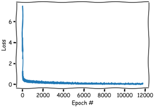
对训练误差进行可视化:
模型在测试集的准确率如下所示:
cnn.eval()
correct = 0
total = 0
for images, labels in test_loader:
    images = images.float().to(device)
    outputs = cnn(images).cpu()
    _, predicted = torch.max(outputs.data, 1)
    total += labels.size(0)
    correct += (predicted == labels).sum()

print('CNN 测试集准确率:%.2f %%' % (100 * correct / total))
# 输出:CNN 测试集准确率:90.78 %
5、优化
修改学习率和批次
cnn.train()
LR = LR / 10
EPOCHES = 20
optimizer = torch.optim.Adam(cnn.parameters(), lr=LR)
losses = []
for epoch in range(EPOCHES):
    for i, (images, labels) in enumerate(train_loader):
        images = images.float().to(device)
        labels = labels.to(device)
        optimizer.zero_grad()
        outputs = cnn(images)
        loss = criterion(outputs, labels).cpu()
        loss.backward()
        optimizer.step()
        losses.append(loss.data.item())
        if (i + 1) % 100 == 0:
            print('Epoch : %d/%d, Iter : %d/%d, Loss : %.4f' % (
                epoch + 1, EPOCHES,
                i + 1, len(train_dataset) // BATCH_SIZE,
                loss.data.item()
            ))
优化后的训练输出如下所示:
Epoch : 1/20, Iter : 100/234, Loss : 0.0042
Epoch : 1/20, Iter : 200/234, Loss : 0.0055
Epoch : 2/20, Iter : 100/234, Loss : 0.0027
Epoch : 2/20, Iter : 200/234, Loss : 0.0016
Epoch : 3/20, Iter : 100/234, Loss : 0.0040
Epoch : 3/20, Iter : 200/234, Loss : 0.0035
Epoch : 4/20, Iter : 100/234, Loss : 0.0010
Epoch : 4/20, Iter : 200/234, Loss : 0.0015
Epoch : 5/20, Iter : 100/234, Loss : 0.0009
Epoch : 5/20, Iter : 200/234, Loss : 0.0013
......
Epoch : 15/20, Iter : 100/234, Loss : 0.0004
Epoch : 15/20, Iter : 200/234, Loss : 0.0002
Epoch : 16/20, Iter : 100/234, Loss : 0.0005
Epoch : 16/20, Iter : 200/234, Loss : 0.0007
Epoch : 17/20, Iter : 100/234, Loss : 0.0002
Epoch : 17/20, Iter : 200/234, Loss : 0.0003
Epoch : 18/20, Iter : 100/234, Loss : 0.0003
Epoch : 18/20, Iter : 200/234, Loss : 0.0001
Epoch : 19/20, Iter : 100/234, Loss : 0.0009
Epoch : 19/20, Iter : 200/234, Loss : 0.0002
Epoch : 20/20, Iter : 100/234, Loss : 0.0002
Epoch : 20/20, Iter : 200/234, Loss : 0.0001
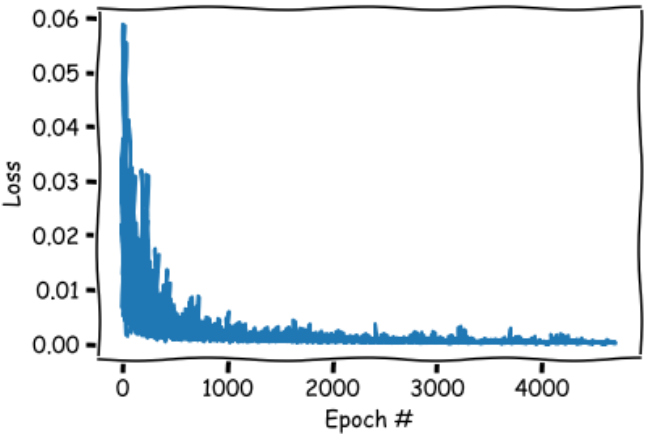
对优化的训练误差进行可视化:
优化后的模型在测试集的准确率如下所示(91.89%):
cnn.eval()
correct = 0
total = 0
for images, labels in test_loader:
    images = images.float().to(device)
    outputs = cnn(images).cpu()
    _, predicted = torch.max(outputs.data, 1)
    total += labels.size(0)
    correct += (predicted == labels).sum()

print('CNN 测试集准确率:%.2f %%' % (100 * correct / total))
# CNN 测试集准确率:91.89 %
三、总结
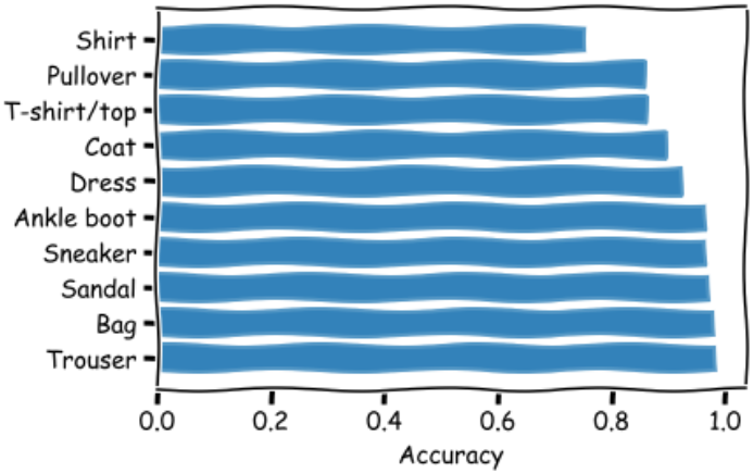
本文通过构建卷积神经网络模型,对Fashion-MNIST图片数据进行分类,优化后的分类效果达到91.89%。当前模型以达到了瓶颈,无法进一步提升准确率,若想提升分类的准确率,可采用更复杂的模型架构,或加深模型的深度。通过细分预测结果,得出准确率在90%以下的类别:T-shirt/top、Pullover、Shirt,其中Shirt的准确率仅为75%。

 浙公网安备 33010602011771号