


1.根据某个列进行groupby,判断是否存在重复列。
# Count the unique variables (if we got different weight values,
# for example, then we should get more than one unique value in this groupby)
all_cols_unique_players = df.groupby('playerShort').agg({col:'nunique' for col in player_cols})
其中针对.agg函数:
DataFrame.agg(self, func, axis=0, *args, **kwargs)[source]
Aggregate using one or more operations over the specified axis.
例子:
>>> df = pd.DataFrame([[1, 2, 3],
...                    [4, 5, 6],
...                    [7, 8, 9],
...                    [np.nan, np.nan, np.nan]],
...                   columns=['A', 'B', 'C'])


>>> df.agg({'A' : ['sum', 'min'], 'B' : ['min', 'max']})
        A    B
max   NaN  8.0
min   1.0  2.0
sum  12.0  NaN
2.获取一个字表
其主要实现的是: """Helper function that creates a sub-table from the columns and runs a quick uniqueness test."""
player_index = 'playerShort'
player_cols = [#'player', # drop player name, we have unique identifier
               'birthday',
               'height',
               'weight',
               'position',
               'photoID',
               'rater1',
               'rater2',
              ]
def get_subgroup(dataframe, g_index, g_columns):
    """Helper function that creates a sub-table from the columns and runs a quick uniqueness test."""
    g = dataframe.groupby(g_index).agg({col:'nunique' for col in g_columns})
    if g[g > 1].dropna().shape[0] != 0:
        print("Warning: you probably assumed this had all unique values but it doesn't.")
    return dataframe.groupby(g_index).agg({col:'max' for col in g_columns})
players = get_subgroup(df, player_index, player_cols)
players.head()
3.将整理出的字表存储至CSV文件
def save_subgroup(dataframe, g_index, subgroup_name, prefix='raw_'):
    save_subgroup_filename = "".join([prefix, subgroup_name, ".csv.gz"])
    dataframe.to_csv(save_subgroup_filename, compression='gzip', encoding='UTF-8')
    test_df = pd.read_csv(save_subgroup_filename, compression='gzip', index_col=g_index, encoding='UTF-8')
    # Test that we recover what we send in
    if dataframe.equals(test_df):
        print("Test-passed: we recover the equivalent subgroup dataframe.")
    else:
        print("Warning -- equivalence test!!! Double-check.")
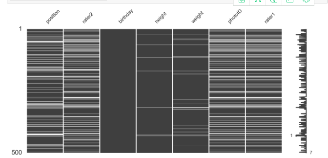
4.数据具体指标查看---缺失值查看
import missingno as msno
import pandas_profiling
msno.matrix(players.sample(500),
            figsize=(16, 7),
            width_ratios=(15, 1))
msno.heatmap(players.sample(500),
            figsize=(16, 7),)

5.数据透视表
转至https://blog.csdn.net/Dorisi_H_n_q/article/details/82288092
透视表概念:pd.pivot_table()
透视表是各种电子表格程序和其他数据分析软件中一种常见的数据汇总工具。它根据一个或多个键对数据进行聚合,并根据行和列上的分组键将数据分配到各个矩形区域中。
 透视表:根据特定条件进行分组计算,查找数据,进行计算
pd.pivot_table(df,index=['hand'],columns=['male'],aggfunc='min')
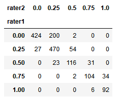
交叉表概念:pd.crosstab(index,colums)
交叉表是一种用于计算分组频率的特殊透视图,对数据进行汇总。
pd.crosstab(players.rater1, players.rater2)
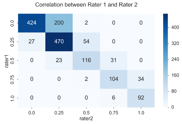
fig, ax = plt.subplots(figsize=(12, 8))
sns.heatmap(pd.crosstab(players.rater1, players.rater2), cmap='Blues', annot=True, fmt='d', ax=ax)
ax.set_title("Correlation between Rater 1 and Rater 2\n")
fig.tight_layout()
创建一个新列,新列的值是另外两列的平均值
players['skintone'] = players[['rater1', 'rater2']].mean(axis=1)
players.head()
6.对离散category数值进行处理
#连续变量离散化
weight_categories = ["vlow_weight",
                     "low_weight",
                     "mid_weight",
                     "high_weight",
                     "vhigh_weight",
                    ]

players['weightclass'] = pd.qcut(players['weight'],
                                 len(weight_categories),
                                 weight_categories)
(Create higher level categories)
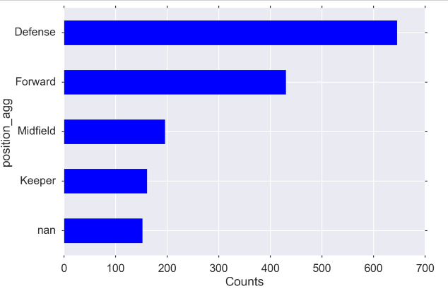
position_types = players.position.unique()
position_types
“”“
array(['Center Back', 'Attacking Midfielder', 'Right Midfielder',
       'Center Midfielder', 'Goalkeeper', 'Defensive Midfielder',
       'Left Fullback', nan, 'Left Midfielder', 'Right Fullback',
       'Center Forward', 'Left Winger', 'Right Winger'], dtype=object)
”“”

defense = ['Center Back','Defensive Midfielder', 'Left Fullback', 'Right Fullback', ]
midfield = ['Right Midfielder', 'Center Midfielder', 'Left Midfielder',]
forward = ['Attacking Midfielder', 'Left Winger', 'Right Winger', 'Center Forward']
keeper = 'Goalkeeper'

# modifying dataframe -- adding the aggregated position categorical position_agg
players.loc[players['position'].isin(defense), 'position_agg'] = "Defense"
players.loc[players['position'].isin(midfield), 'position_agg'] = "Midfield"
players.loc[players['position'].isin(forward), 'position_agg'] = "Forward"
players.loc[players['position'].eq(keeper), 'position_agg'] = "Keeper"
绘制value_counts()图片
MIDSIZE = (12, 8)
fig, ax = plt.subplots(figsize=MIDSIZE)
players['position_agg'].value_counts(dropna=False, ascending=True).plot(kind='barh', ax=ax)
ax.set_ylabel("position_agg")
ax.set_xlabel("Counts")
fig.tight_layout()
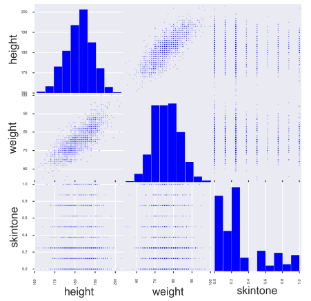
7.绘制多变量之间的关系图
from pandas.plotting import scatter_matrix
fig, ax = plt.subplots(figsize=(10, 10))
scatter_matrix(players[['height', 'weight', 'skintone']], alpha=0.2, diagonal='hist', ax=ax);
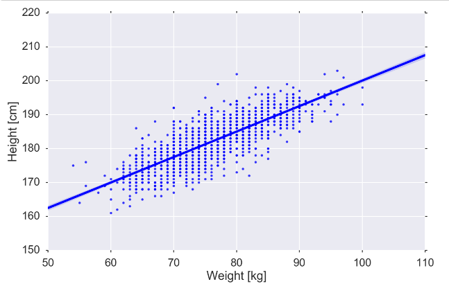
# Perhaps you want to see a particular relationship more clearly
fig, ax = plt.subplots(figsize=MIDSIZE)
sns.regplot('weight', 'height', data=players, ax=ax)
ax.set_ylabel("Height [cm]")
ax.set_xlabel("Weight [kg]")
fig.tight_layout()
8.连续变量离散化(Create quantile bins for continuous variables)
weight_categories = ["vlow_weight",
                     "low_weight",
                     "mid_weight",
                     "high_weight",
                     "vhigh_weight",
                    ]

players['weightclass'] = pd.qcut(players['weight'],
                                 len(weight_categories),
                                 weight_categories)
9.数据报表查看
pandas_profiling.ProfileReport(players)

10.出生日期等时间格式处理
players['birth_date'] = pd.to_datetime(players.birthday, format='%d.%m.%Y')
players['age_years'] = ((pd.to_datetime("2013-01-01") - players['birth_date']).dt.days)/365.25
players['age_years']
//选择特定列
players_cleaned_variables = players.columns.tolist()
players_cleaned_variables
player_dyad = (clean_players.merge(agg_dyads.reset_index().set_index('playerShort'),
                                   left_index=True,
                                   right_index=True))
//groupby+sort_values+rename
(tidy_dyads.groupby(level=1)
           .sum()
           .sort_values('redcard', ascending=False)
           .rename(columns={'redcard':'total redcards received'})).head()
针对时间统计可以分别列出,年、月、日以及相应的小时等数据,查看年的、月的、季度的、每天时间段的各个统计量。
11.数据偏度与峰度
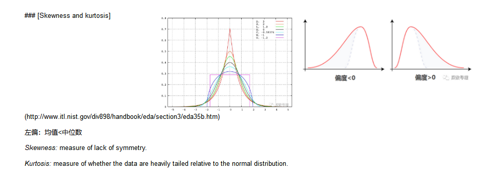
正态分布的偏度应为零。负偏度表示偏左,正偏表示右偏。
峰度也是一个正态分布和零只能是积极的。我们肯定有一些异常值!
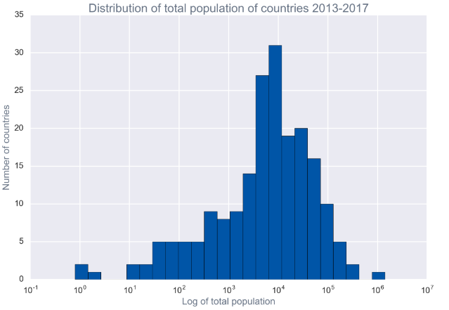
对于分布超级不均衡的数据,采用log变换的方式,将变量的统计部分变为正常。
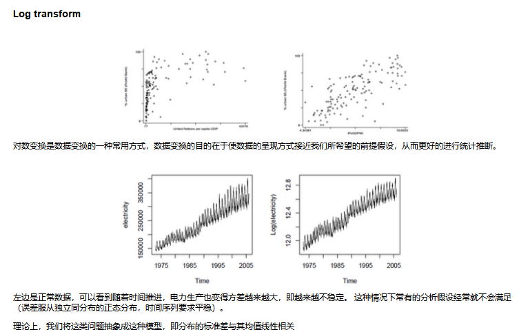
具体的代码采用的是np.log
recent[['total_pop']].apply(np.log).apply(scipy.stats.skew)
//绘图函数
def plot_hist(df, variable, bins=20, xlabel=None, by=None,
              ylabel=None, title=None, logx=False, ax=None):

    if not ax:
        fig, ax = plt.subplots(figsize=(12,8))
    if logx:
        if df[variable].min() <=0:
            df[variable] = df[variable] - df[variable].min() + 1
            print('Warning: data <=0 exists, data transformed by %0.2g before plotting' % (- df[variable].min() + 1))

        bins = np.logspace(np.log10(df[variable].min()),
                           np.log10(df[variable].max()), bins)
        ax.set_xscale("log")

    ax.hist(df[variable].dropna().values, bins=bins);

    if xlabel:
        ax.set_xlabel(xlabel);
    if ylabel:
        ax.set_ylabel(ylabel);
    if title:
        ax.set_title(title);

    return ax
plot_hist(recent, 'total_pop', bins=25, logx=True,
          xlabel='Log of total population', ylabel='Number of countries',
          title='Distribution of total population of countries 2013-2017');

查看单个变量之间的变化规律时,在出现变量数值不均衡,有的数值很大,有的很小时,可以采用变量的增长速度比率进行表示,查看其变化情况。例子:
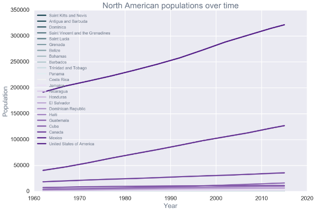
原数据
with sns.color_palette(sns.diverging_palette(220, 280, s=85, l=25, n=23)):
    north_america = time_slice(subregion(data, 'North America'), '1958-1962').sort_values('total_pop').index.tolist()
    for country in north_america:
        plt.plot(time_series(data, country, 'total_pop'), label=country);
        plt.xlabel('Year');
        plt.ylabel('Population');
        plt.title('North American populations over time');
    plt.legend(loc=2,prop={'size':10});
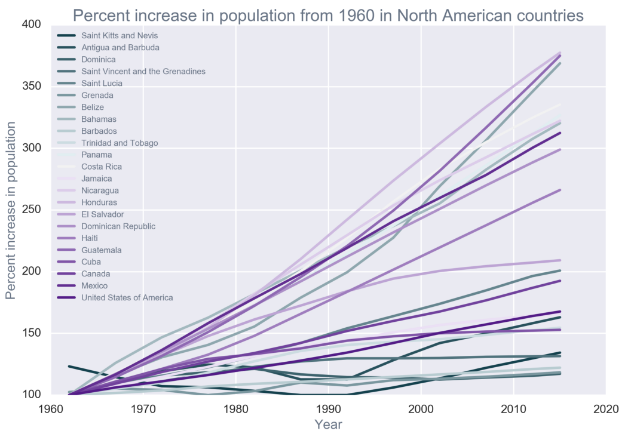
比率处理后的数据可视化
with sns.color_palette(sns.diverging_palette(220, 280, s=85, l=25, n=23)):
    for country in north_america:
        ts = time_series(data, country, 'total_pop')
        ts['norm_pop'] = ts.total_pop/ts.total_pop.min()*100
        plt.plot(ts['norm_pop'], label=country);
        plt.xlabel('Year');
        plt.ylabel('Percent increase in population');
        plt.title('Percent increase in population from 1960 in North American countries');
        plt.legend(loc=2,prop={'size':10});
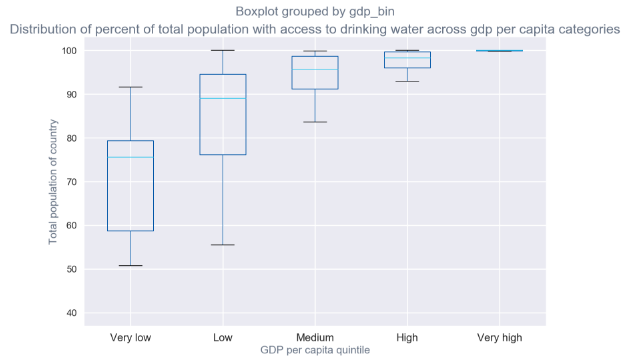
recent[['gdp_bin','total_pop_access_drinking']].boxplot(by='gdp_bin');
# plt.ylim([0,100000]);
plt.title('Distribution of percent of total population with access to drinking water across gdp per capita categories');
plt.xlabel('GDP per capita quintile');
plt.ylabel('Total population of country');
12.对特定列进行处理
simple_regions ={
    'World | Asia':'Asia',
    'Americas | Central America and Caribbean | Central America': 'North America',
    'Americas | Central America and Caribbean | Greater Antilles': 'North America',
    'Americas | Central America and Caribbean | Lesser Antilles and Bahamas': 'North America',
    'Americas | Northern America | Northern America': 'North America',
    'Americas | Northern America | Mexico': 'North America',
    'Americas | Southern America | Guyana':'South America',
    'Americas | Southern America | Andean':'South America',
    'Americas | Southern America | Brazil':'South America',
    'Americas | Southern America | Southern America':'South America',
    'World | Africa':'Africa',
    'World | Europe':'Europe',
    'World | Oceania':'Oceania'
}
data.region = data.region.apply(lambda x: simple_regions[x])

 浙公网安备 33010602011771号