
scrapy爬取豆瓣电影+可视化分析
项目介绍
本项目用于大数据分析大作业,使用scrapy爬取豆瓣电影历史top500,以及2016-2021每年豆瓣电影top500,使用pycharts可视化分析。本文具体说明分析结果。
scrapy爬取豆瓣电影
scrapy爬取豆瓣电影历史top500
豆瓣电影中并无专门网址显示历史top500电影,我认为豆瓣电影排名可以基于某种标签进行分类,最后选择如下网页网址进行爬取。
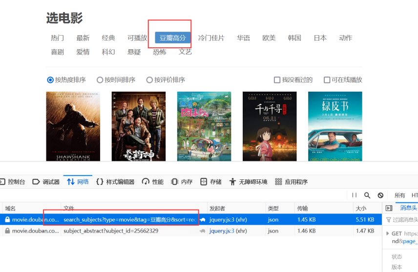
实现逻辑
- 先爬取top500的每部电影id与电影名,保存为字典。网址如上,是通过ajax发送,每页有20个电影。
- 通过遍历之前保存的电影id与电影名字典,拼接成每部电影的详情页url,通过yield Request生成新的请求。
- 通过指定的callback接收新的请求,对电影详情页进行处理,获取我们想要的信息,形成item
- 在pipeline.py中,设置输出csv文件
MovieSpider.py主要代码
class MovieSpider(scrapy.Spider):
    name="doubanMovie"
    allowed_domains = ["movie.douban.com"]
    movie_sum=500
    movie_tag='豆瓣高分'
    movies_id_and_title_dict = {}

    #设置起始链接
    def start_requests(self):
        """
        获取影片名和影片ID
        :param movie_sum: 指定爬取电影的数量,范围 1~500
        :param movie_tag: 指定电影排行tag, 范围 '热门' or '豆瓣高分'
        :return:
        """
        movie_tags = {'热门': '%E7%83%AD%E9%97%A8', '豆瓣高分': '%E8%B1%86%E7%93%A3%E9%AB%98%E5%88%86'}
        tag = movie_tags[self.movie_tag]
        print('====================>> Start time: ' + get_current_time() + ' <<====================')
        print('========================>> 共' + str(self.movie_sum) + ' 部影片 <<========================')

        for i in range(0, self.movie_sum, 20):
            hot_page_url = 'https://movie.douban.com/j/search_subjects?type=movie&tag=' + tag + '&sort=recommend' \
                        '&page_limit=20' + '&page_start=' + str(i)
            try:
                response = get_source_page(hot_page_url)
                result = response.json()['subjects']  # type: list
                response.close()
            except Exception as e:
                print(get_current_time() + '===========>> 正在重试...')
                result = get_source_page(hot_page_url).json()['subjects']  # type: list

            for each_movie in result:
                self.movies_id_and_title_dict[each_movie['id']] = each_movie['title']
                # print(host_movies_id_and_title)

            for mid, mtitle in self.movies_id_and_title_dict.items():
                print(mid + ' --> ' + mtitle)

        # 爬取详细信息
        all_movie_urls = ['https://movie.douban.com/subject/{}/'.format(k) for k, v in self.movies_id_and_title_dict.items()]
        movies_all = []
        sum = 1
        for each_page in all_movie_urls:
            movie_id = each_page.split('/')[-2]
            print(get_current_time() + ' ----->> 正在爬取第 ' + str(sum) + '部影片( ' + self.movies_id_and_title_dict[movie_id] + ' )')

            item = MovieInfoItem()  # 实例化电影详情
            item['orderNum'] =sum  # 排名
            item['movie_id'] = movie_id  # 电影id

            sum += 1

            sleepTime = random.randint(1, 10)
            time.sleep(sleepTime)
            yield Request(each_page,headers=header, cookies=cookies,callback=self.get_movie_info,meta={'item':item})

    #爬取详细信息
    def get_movie_info(self,response):

        eachMovie = etree.HTML(response.text)
        movie_info = []
        # movie_id = movie_id
        movie_name = eachMovie.xpath('//span[@property="v:itemreviewed"]/text()')[0]  # 电影名
        release_year = eachMovie.xpath('//span[@class="year"]/text()')[0].strip('()')  # 年份
        director = eachMovie.xpath('//div[@id="info"]/span[1]/span[@class="attrs"]/a/text()')[0]  # 导演
        starring = eachMovie.xpath('//span[@class="actor"]//span[@class="attrs"]/a/text()')  # 主演
        starring = "/".join(starring)
        genre = eachMovie.xpath('//span[@property="v:genre"]/text()')  # 类型
        genre = "/".join(genre)
        info = eachMovie.xpath('//div[@id="info"]//text()')
        for i in range(0, len(info)):
            if str(info[i]).find('语言') != -1:
                languages = info[i + 1].strip()  # 语言
            if str(info[i]).find('制片国家') != -1:
                country = info[i + 1].strip()  # 国别
        country = country
        languages = languages
        rating_num = eachMovie.xpath('//strong[@property="v:average"]/text()')[0]  # 评分
        vote_num = eachMovie.xpath('//span[@property="v:votes"]/text()')[0]  # 评分人数
        rating_per_stars5 = eachMovie.xpath('//span[@class="rating_per"]/text()')[0]  # 五星占比,四星占比,三星占比,二星占比,一星占比
        rating_per_stars4 = eachMovie.xpath('//span[@class="rating_per"]/text()')[1]
        rating_per_stars3 = eachMovie.xpath('//span[@class="rating_per"]/text()')[2]
        rating_per_stars2 = eachMovie.xpath('//span[@class="rating_per"]/text()')[3]
        rating_per_stars1 = eachMovie.xpath('//span[@class="rating_per"]/text()')[4]
        introduction = eachMovie.xpath('//span[@property="v:summary"]/text()')[0].strip()  # 简介
        comment_num = eachMovie.xpath('//div[@id="comments-section"]/div[@class="mod-hd"]/h2//a/text()')[0]  # 短评数
        comment_num = re.findall('\d+', comment_num)[0]
        item= response.meta["item"]
        item['movie_name']=movie_name
        item['release_year'] = release_year
        item['director'] = director
        item['starring'] = starring
        item['genre'] = genre
        item['languages'] = languages
        item['country']=country
        item['rating_num'] = rating_num
        item['vote_num'] = vote_num
        item['rating_per_stars5'] = rating_per_stars5
        item['rating_per_stars4'] = rating_per_stars4
        item['rating_per_stars3'] = rating_per_stars3
        item['rating_per_stars2'] = rating_per_stars2
        item['rating_per_stars1'] = rating_per_stars1
        item['introduction'] = introduction
        item['comment_num'] = comment_num

        yield item
scrapy爬取2016-2021年豆瓣电影top500
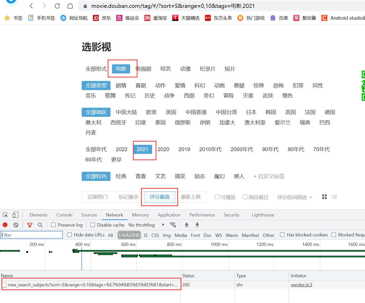
豆瓣电影中并无专门网址显示2016-2021年豆瓣top500电影,同历史Top500一样认为是基于某种标签进行分类,最后选择如下网页网址进行爬取。
实现逻辑
- 按年份爬取当年的top500的每部电影id与电影名,保存为字典。是通过ajax发送,每页有20个电影。
- 通过遍历之前保存的电影id与电影名字典,拼接成每部电影的详情页url,通过yield Request生成新的请求。
- 通过指定的callback接收新的请求,对电影详情页进行处理,获取我们想要的信息,形成item.
- 在pipeline.py中,设置输出csv文件
- 最终的到的结果为6个csv文件
因为豆瓣电影反爬比较严格,代码中采取按年爬取,每次爬取100个电影。运行时仅需要修改MovieSpider.py中years数组以及movie_sum电影数即可
MovieSpider.py主要代码
class MovieSpider(scrapy.Spider):
    name = 'movie2016_2021'
    allowed_domains = ["movie.douban.com"]
    movie_sum = 500  #电影数
    year=""         #当前爬取的年份

    movies_id_and_title_dict = {}


    #设置起始链接
    def start_requests(self):
        """
        获取影片名和影片ID
        :param movie_sum: 指定爬取电影的数量,范围 1~500
        :param movie_tag: 指定电影排行tag, 范围 '热门' or '豆瓣高分'
        :return:
        """
        print('====================>> Start time: ' + get_current_time() + ' <<====================')
        print('========================>> 共' + str(self.movie_sum) + ' 部影片 <<========================')
        years = [2021]
        #, 2017, 2018, 2019, 2020, 2021
        for j in years:
            self.year = str(j)
            self.movies_id_and_title_dict={}
            for i in range(0, self.movie_sum, 20):
                sleepTime = random.randint(1, 5)
                time.sleep(sleepTime)
                hot_page_url = 'https://movie.douban.com/j/new_search_subjects?sort=S&range=0,10&tags=%E7%94%B5%E5%BD%B1&start='+str(i)+'&year_range=' + str(j) + "," + str(j)
                try:
                    response = requests.get(hot_page_url, headers=headers)

                except Exception as e:
                    print(get_current_time() + '===========>> 正在重试...'+e)
                    response = requests.get(hot_page_url, headers=headers)

                result = response.json()['data']  # type: list
                response.close()
                for each_movie in result:
                    self.movies_id_and_title_dict[each_movie['id']] = each_movie['title']
                    # print(host_movies_id_and_title)

                for mid, mtitle in self.movies_id_and_title_dict.items():
                    print(mid + ' --> ' + mtitle)

            # 爬取详细信息
            all_movie_urls = ['https://movie.douban.com/subject/{}/'.format(k) for k, v in self.movies_id_and_title_dict.items()]
            movies_all = []
            sum = 1
            for each_page in all_movie_urls:
                movie_id = each_page.split('/')[-2]
                print(get_current_time() + ' ----->> 正在爬取第 ' + str(sum) + '部影片( ' + self.movies_id_and_title_dict[movie_id] + ' )')

                item = MovieInfoItem()  # 实例化电影详情
                item['orderNum'] = sum # 排名
                item['movie_id'] = movie_id  # 电影id

                sum += 1

                sleepTime = random.randint(1, 10)
                time.sleep(sleepTime)
                yield Request(each_page,headers=header,cookies=cookies,callback=self.get_movie_info,meta={'item':item})

    #爬取详细信息
    def get_movie_info(self,response):

        eachMovie = etree.HTML(response.text)
        movie_info = []
        # movie_id = movie_id
        movie_name = eachMovie.xpath('//span[@property="v:itemreviewed"]/text()')[0]  # 电影名
        movie_name.replace(',',' ') #名称里面可能含有",",转换为csv时可能出错
        release_year = eachMovie.xpath('//span[@class="year"]/text()')[0].strip('()')  # 年份
        director = eachMovie.xpath('//div[@id="info"]/span[1]/span[@class="attrs"]/a/text()')[0]  # 导演
        starring = eachMovie.xpath('//span[@class="actor"]//span[@class="attrs"]/a/text()')  # 主演
        starring = "/".join(starring)
        genre = eachMovie.xpath('//span[@property="v:genre"]/text()')  # 类型
        genre = "/".join(genre)
        info = eachMovie.xpath('//div[@id="info"]//text()')
        for i in range(0, len(info)):
            if str(info[i]).find('语言') != -1:
                languages = info[i + 1].strip()  # 语言
            if str(info[i]).find('制片国家') != -1:
                country = info[i + 1].strip()  # 国别
        country = country
        languages = languages
        rating_num = eachMovie.xpath('//strong[@property="v:average"]/text()')[0]  # 评分
        vote_num = eachMovie.xpath('//span[@property="v:votes"]/text()')[0]  # 评分人数
        rating_per_stars5 = eachMovie.xpath('//span[@class="rating_per"]/text()')[0]  # 五星占比,四星占比,三星占比,二星占比,一星占比
        rating_per_stars4 = eachMovie.xpath('//span[@class="rating_per"]/text()')[1]
        rating_per_stars3 = eachMovie.xpath('//span[@class="rating_per"]/text()')[2]
        rating_per_stars2 = eachMovie.xpath('//span[@class="rating_per"]/text()')[3]
        rating_per_stars1 = eachMovie.xpath('//span[@class="rating_per"]/text()')[4]
        comment_num = eachMovie.xpath('//div[@id="comments-section"]/div[@class="mod-hd"]/h2//a/text()')[0]  # 短评数
        comment_num = re.findall('\d+', comment_num)[0]

        item= response.meta["item"]
        item['movie_name']=movie_name
        item['release_year'] = release_year
        item['director'] = director
        item['starring'] = starring
        item['genre'] = genre
        item['languages'] = languages
        item['country']=country
        item['rating_num'] = rating_num
        item['vote_num'] = vote_num
        item['rating_per_stars5'] = rating_per_stars5
        item['rating_per_stars4'] = rating_per_stars4
        item['rating_per_stars3'] = rating_per_stars3
        item['rating_per_stars2'] = rating_per_stars2
        item['rating_per_stars1'] = rating_per_stars1
        item['comment_num'] = comment_num

        yield item
爬取电影评论
这里仅爬取几部电影的评论,为2016-2021年top500与历史top500中重合的电影。并按评分进行排序,取前10;按评论人数进行排序取前10;按短评数排序取前10;最后取交集,得到最终结果有6部电影。
爬取一个电影的评论,评论网址如下,评论可通过地址变化得到。

实现逻辑
- 设定6部电影的电影Id与电影名字典。
- 通过遍历之前保存的电影id与电影名字典,爬取每部电影前200条评论,每页20个。并通过start参数的增长,拼接成每部电影的评论url
- 通过指定的callback接收新的请求,对每部电影的每页评论爬取,获取我们想要的信息,形成item.
- 在pipeline.py中,设置输出csv文件
- 最终的到的结果为6个电影评论的csv文件
Comment.py主要代码
class MovieCommentSpider(scrapy.Spider):
    name = "MovieComment"
    allowed_domains = ["movie.douban.com"]
    movies_id_and_title_dict = {'25662329': '疯狂动物城 Zootopia', '26387939': '摔跤吧!爸爸 Dangal',
                           '26580232': '看不见的客人 Contratiempo',
                           '25986180': '釜山行 부산행', '26325320': '血战钢锯岭 Hacksaw Ridge',
                           '25980443': '海边的曼彻斯特 Manchester by the Sea'}
    # movies_id_and_title_dict={'26387939': '摔跤吧!爸爸 Dangal'}

    # 设置起始链接
    def start_requests(self):
        number = 1
        for movie_id, movie_name in self.movies_id_and_title_dict.items():
            print(' ----->> 正在爬取第 ' + str(number) + '部影片( ' + movie_name + ' )')
            base_url = 'https://movie.douban.com/subject/' + str(movie_id) + '/comments?start={}&limit=20&status=P&sort=new_score'
            number += 1
            all_page_comments = [base_url.format(x) for x in range(0, 201, 20)]

            for each_page in all_page_comments:

                item=CommentItem()
                item['title']=movie_name
                time.sleep(random.randint(1,10))
                yield Request(url=each_page,meta={"item":item},callback=self.getComment,headers=headers)


    #得到电影评论
    def getComment(self,response):
        html = response
        selector = etree.HTML(html.text)
        comments = selector.xpath("//div[@class='comment']")
        for eachComment in comments:

            user = eachComment.xpath("./h3/span[@class='comment-info']/a/text()")[0]  # 用户
            watched = eachComment.xpath("./h3/span[@class='comment-info']/span[1]/text()")[0]  # 是否看过
            rating = eachComment.xpath("./h3/span[@class='comment-info']/span[2]/@title")  # 五星评分
            if len(rating) > 0:
                rating = rating[0]

            comment_time = eachComment.xpath("./h3/span[@class='comment-info']/span[3]/@title")  # 评论时间
            if len(comment_time) > 0:
                comment_time = comment_time[0]
            else:
                comment_time = ' '

            votes = eachComment.xpath("./h3/span[@class='comment-vote']/span/text()")[0]  # "有用"数
            content = eachComment.xpath("./p/span/text()")[0].strip()  # 评论内容

            item= response.meta["item"]
            item['user']=user
            item['watched']=watched
            item['rating']=rating
            item['votes'] = votes
            item['comment_time'] = comment_time
            item['content'] = content
            yield item
可视化分析
对2016-2021年top500电影按国别进行统计发行量
def make_geo_map(self):
"""
生成世界地图,根据各国电影发行量
:return:
"""
# 对2016-2021数据进行去空去重
excel_path = '../kettle/2016-2021/file2016-2021.xls'
rows = pd.read_excel(io=excel_path, sheet_name=0, header=0)
# 去空
rows.dropna(axis=0, how='any', inplace=True) # axis=0表示index行 "any"表示这一行或列中只要有元素缺失,就删除这一行或列
# 移除重复行
rows.drop_duplicates(subset=['电影id'], keep='first',
inplace=True) # subset参数是一个列表,这个列表是需要你填进行相同数据判断的条件 keep=first时,保留相同数据的第一条。。inplace=True时,会对原数据进行修改。
# 分析并统计数据
res = rows['国别'].to_frame()
# 数据分割
country_list = []
for i in res.itertuples():
for j in i[1].split('/'):
country_list.append(j)
# 数据统计
df = pd.DataFrame(country_list, columns=['国别'])
res = df.groupby('国别')['国别'].count().sort_values(ascending=False)
raw_data = [i for i in res.items()]
# 导入映射数据,英文名 -> 中文名
country_name = pd.read_json('countries_zh_to_en.json', orient='index')
stand_data = [i for i in country_name[0].items()]
# 数据转换
res_code = {}
for raw_country in raw_data:
for stand_country in stand_data:
if stand_country[1] in raw_country[0]:
if (stand_country[0]) in res_code.keys():
res_code[stand_country[0]] += raw_country[1]
else:
res_code[stand_country[0]] = raw_country[1]
d_order = sorted(res_code.items(), key=lambda x: x[1], reverse=True) # 按字典集合中,每一个元组的第二个元素排列。# x相当于字典集合中遍历出来的一个元组。
data = []
for i in d_order:
data.append([i[0],i[1]])
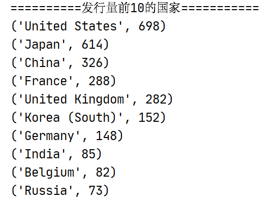
print("==========发行量前10的国家===========")
for i in range(10):
print(d_order[i])
# 制作图表
c = Map()
c.add("电影发行量", data, "world") # 世界地图
c.set_series_opts(label_opts=opts.LabelOpts(is_show=False)) # 显示标签
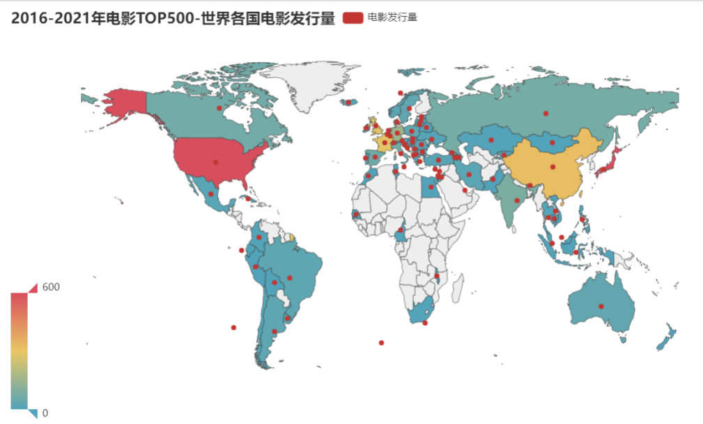
c.set_global_opts(title_opts=opts.TitleOpts(title="2016-2021年电影TOP500-世界各国电影发行量"),
visualmap_opts=opts.VisualMapOpts(
max_=600)) # VisualMapOpts:视觉映射配置项,用于显示图例,max_ # 指定 visualMapPiecewise 组件的最大值。
# 生成html
#c.render("世界各国电影发行量.html")
return c
运行结果
分析
可以发现美国,日本,中国,法国的电影发行量处于前四。
结合电影发行量前10的国家与地图中可以看出这些国家多分布在北美洲,欧洲,东亚地区。结合前十中欧美国家的电影发行量(1416)与东亚地区(1092)可以得出,欧美电影与东亚电影在世界电影市场中占主流。
分析中美两国2016-2021年同时间段内Top500豆瓣电影
中美电影产量对比
#2016-2021年中美两国产量对比
def make_line_AmericanAndChina(self):
#对2016-2021数据进行去空去重
excel_path='../kettle/2016-2021/file2016-2021.xls'
rows=pd.read_excel(io=excel_path,sheet_name=0,header=0)
# 去空
rows.dropna(axis=0,how='any',inplace=True) #axis=0表示index行 "any"表示这一行或列中只要有元素缺失,就删除这一行或列
# 移除重复行
rows.drop_duplicates(subset=['电影id'],keep='first',inplace=True) #subset参数是一个列表,这个列表是需要你填进行相同数据判断的条件 keep=first时,保留相同数据的第一条。。inplace=True时,会对原数据进行修改。
# #统计空值
# print(rows.isnull().sum())
# print("--------------------------------------")
# # 统计重复值
# dup = rows[rows.duplicated()].count()
# print(dup)
to_drop = ['电影id', '名称', '导演', '演员', '语言','类型', '评分', '评分人数', '五星占比', '四星占比', '三星占比', '二星占比',
'一星占比', '短评数']
res = rows.drop(to_drop, axis=1)
# 数据统计
American_dict = {}
China_dict={}
for i in res.itertuples(): #将DataFrame迭代为元祖。
if '美国' in i[2]:
if str(i[1]) in American_dict.keys():
American_dict[str(i[1])] += 1
else:
American_dict[str(i[1])]=1
if '中国大陆' in i[2] or '中国香港' in i[2] or '中国台湾' in i[2] or '中国澳门' in i[2]:
if str(i[1]) in China_dict.keys():
China_dict[str(i[1])] += 1 #发行量+1
else:
China_dict[str(i[1])]=1 #新建
print("=======美国==========")
print(American_dict)
print("=======中国===========")
print(China_dict)
American_list=[]
for k,v in American_dict.items():
American_list.append(v)
China_list=[]
for k,v in China_dict.items():
China_list.append(v)
years=['2016','2017','2018','2019','2020','2021']
# 制作图表
c = Line()
c.add_xaxis(years)
c.add_yaxis("美国发行电影数量", American_list)
c.add_yaxis("中国发行电影数量", China_list, color=Faker.rand_color())
c.set_global_opts(
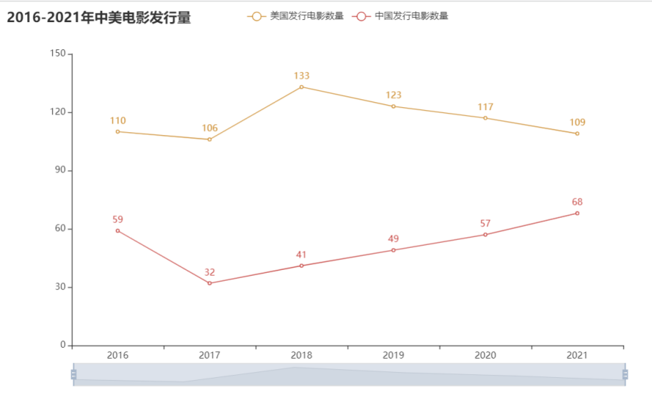
title_opts=opts.TitleOpts(title="2016-2021年中美电影发行量"),
datazoom_opts=[opts.DataZoomOpts(), opts.DataZoomOpts(type_="inside")],
)
# 生成html
#c.render("2016-2021中美电影发行量.html")
return c
运行结果
分析
可以看出在电影产量上美国在各个时间内都超过中国, 但自2018年后,中国电影发行量上升,美国电影发行量有所下降。
结合历史Top500电影数据进行分析
#历史电影TOP500榜单中 - 各年份电影发行量
def make_relase_year_bar(self):
"""
生成各年份电影发行量柱状图
:return:
"""
to_drop = ['排名', '电影id', '名称', '导演', '演员', '国别', '类型', '语言', '评分', '评分人数', '五星占比', '四星占比', '三星占比', '二星占比',
'一星占比', '短评数',
'简介']
res = self.newRows.drop(to_drop, axis=1)
# 数据分析
res_by = res.groupby('年份')['年份'].count().sort_values(ascending=False)
res_by2 = res_by.sort_index(ascending=False)
type(res_by2)
years = []
datas = []
for k, v in res_by2.items():
years.append(k)
datas.append(v)
# 生成图表
c = Bar()
c.add_xaxis(years)
c.add_yaxis("发行电影数量", datas, color=Faker.rand_color())
c.set_global_opts(
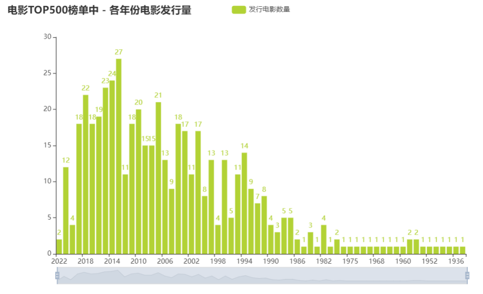
title_opts=opts.TitleOpts(title="历史电影TOP500榜单中 - 各年份电影发行量"),
datazoom_opts=[opts.DataZoomOpts(), opts.DataZoomOpts(type_="inside")],
)
# 生成html
#c.render("各年份电影发行量.html")
return c
运行结果
分析
自2000年后,世界电影发行量增多,在20世纪10年代,世界电影蓬勃发展,发行量达到历史的高峰,中国电影受世界市场的影响而增大了发行量也不足为奇。而自2019年新冠病毒的爆发,对线下电影界的冲击可谓巨大,导致世界电影发行量减少, 而美国作为电影发行量第一的国家,电影发行量也减少。而中国的电影发行量却增多。由此推测中国电影仍充满活力。
美国电影评分与中国电影评分对比
#2016-2021中美评分对比
def make_Boxplot_AmericanAndChina(self):
# 对2016-2021数据进行去空去重
excel_path = '../kettle/2016-2021/file2016-2021.xls'
rows = pd.read_excel(io=excel_path, sheet_name=0, header=0)
# 去空
rows.dropna(axis=0, how='any', inplace=True) # axis=0表示index行 "any"表示这一行或列中只要有元素缺失,就删除这一行或列
# 移除重复行
rows.drop_duplicates(subset=['电影id'], keep='first',
inplace=True) # subset参数是一个列表,这个列表是需要你填进行相同数据判断的条件 keep=first时,保留相同数据的第一条。。inplace=True时,会对原数据进行修改。
# #统计空值
# print(rows.isnull().sum())
# print("--------------------------------------")
# # 统计重复值
# dup = rows[rows.duplicated()].count()
# print(dup)
to_drop = ['电影id', '名称','导演', '演员', '语言', '类型', '评分人数', '五星占比', '四星占比', '三星占比', '二星占比',
'一星占比', '短评数']
res = rows.drop(to_drop, axis=1)
#统计
American_dict = {}
China_dict = {}
for i in res.itertuples(): # 将DataFrame迭代为元祖。
if '美国' in i[2]:
if str(i[1]) not in American_dict.keys():
American_score_list = []
American_score_list.append(i[3]) # 加入评分
American_dict[str(i[1])]=American_score_list
else:
American_score_list.append(i[3]) # 加入评分
if '中国大陆' in i[2] or '中国香港' in i[2] or '中国台湾' in i[2] or '中国澳门' in i[2]:
if str(i[1]) not in China_dict.keys():
China_score_list = []
China_score_list.append(i[3]) # 加入评分
China_dict[str(i[1])] = China_score_list
else:
China_score_list.append(i[3]) # 加入评分
print("==========美国评分============")
print(American_dict)
print("==========中国评分============")
print(China_dict)
American_list=[]
for k,v in American_dict.items():
American_list.append(v)
China_list = []
for k, v in China_dict.items():
China_list.append(v)
#制作图表
years = ['2016', '2017', '2018', '2019', '2020', '2021']
c=Boxplot()
c.add_xaxis(years)
c.add_yaxis("美国评分",c.prepare_data(American_list))
c.add_yaxis("中国评分",c.prepare_data(China_list))
c.set_global_opts(
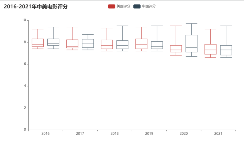
title_opts=opts.TitleOpts(title="2016-2021年中美电影评分"),
)
#生成html
#c.render("2016-2021中美电影评分.html")
return c
运行结果
分析
可以看到生成的盒图中,中位数上中美两国都差不多。集中于7分-8分左右对于豆瓣电影评分10分为满分,而7-8分也属于比较好的得分。而就四分位数,表现为盒子的宽度,美国评分盒子平均较短,评分比较集中 而中国评分在2020年的盒子宽度比较大,评分比较分散,而且中位数靠近盒子底边,评分呈偏右分布,即众数偏小,代表多数评分偏小。 但在2017年时,中国电影评分中位数比美国电影中位数大。
结合2016-2021年中美电影发行量与评分,可以发现中国电影的发行量在提升,且电影评分整体上也不错,但需要关注电影的质量,因为在2020年时电影评分出现比较大的分散。
历史Top500电影分析
分析电影类型占比与数量
根据电影类型生成饼图
#根据电影类型生成饼图
def make_pie_charts(self):
"""
根据电影类型生成饼图
:return:
"""
to_drop = ['排名','电影id','名称', '导演', '演员', '国别', '年份', '语言', '评分', '评分人数', '五星占比', '四星占比', '三星占比', '二星占比', '一星占比', '短评数',
'简介']
res = self.newRows.drop(to_drop, axis=1)
# 数据分割
type_list = []
for i in res.itertuples():
for j in i[1].split('/'):
type_list.append(j)
# 数据统计
df = pd.DataFrame(type_list, columns=['类型'])
res = df.groupby('类型')['类型'].count().sort_values(ascending=False)
res_list = []
for i in res.items():
res_list.append(i)
# 生成饼图
c = Pie()
c.add("", res_list, center=["40%", "55%"], )
c.set_global_opts(
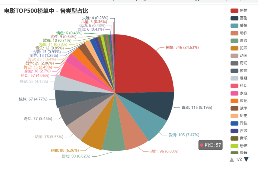
title_opts=opts.TitleOpts(title="历史电影TOP500榜单中 - 各类型占比"),
legend_opts=opts.LegendOpts(type_="scroll", pos_left="80%", orient="vertical"),
)
c.set_series_opts(label_opts=opts.LabelOpts(formatter="{b}: {c} ({d}%)"))
# 生成html
#c.render("各类型占比.html")
return c
生成类型的条形图
#生成类型的条形图
def make_Bar_Types(self):
    to_drop = ['排名', '电影id', '名称', '导演', '演员', '国别', '年份', '语言', '评分', '评分人数', '五星占比', '四星占比', '三星占比', '二星占比',
               '一星占比', '短评数',
               '简介']
    res = self.newRows.drop(to_drop, axis=1)
    # 数据分割
    type_list = []
    for i in res.itertuples():
        for j in i[1].split('/'):
            type_list.append(j)
    # 数据统计
    df = pd.DataFrame(type_list, columns=['类型'])
    res = df.groupby('类型')['类型'].count().sort_values(ascending=False)
    res_list = []
    for i in res.items():
        res_list.append(i)

    #x轴为类型,y轴为数量(下面会反转过来,即y轴为类型,x轴为数量)
    types=[]
    sum=[]
    for i in res_list:
        types.append(i[0])
        sum.append(i[1])

    #生成图表
    c = Bar()

    c.add_xaxis(types)
    c.add_yaxis("电影类型", sum, color=Faker.rand_color())
    c.reversal_axis()
    c.set_series_opts(label_opts=opts.LabelOpts(position="right"))
    c.set_global_opts(
        title_opts=opts.TitleOpts(title="历史电影TOP500榜单中 - 电影类型"),
        # datazoom_opts=[opts.DataZoomOpts(), opts.DataZoomOpts(type_="inside")],
    )
    # 生成html
    #c.render("电影类型.html")

    return c
运行结果
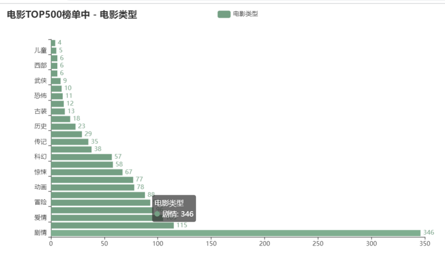
分析
由饼图可以出前三的电影类型为剧情(24.63%)、喜剧(8.19%)、爱情(7.47%)。 随着柱形图可以看到历史top500中电影类型多集中在剧情、喜剧、爱情、动作、冒险、犯罪、动画、奇幻、惊悚、悬疑、科幻。虽然电影的种类由很多,但在历史top500中,由刚刚列出的几项类型占了大多数。
电影类型与评分,评分人数,电影数之间的关系
历史top500电影类型气泡图
#历史top500电影类型气泡图
def make_scatter(self):
    to_drop = ['排名', '电影id', '名称', '导演', '演员', '国别', '年份', '语言',  '五星占比', '四星占比', '三星占比', '二星占比',
               '一星占比',
               '简介']
    res = self.newRows.drop(to_drop, axis=1)
    # 数据分割
    type_dict={}
    for i in res.itertuples():
        for j in i[1].split('/'):
            if j not in type_dict.keys():
                data=[]
                data.append([i[2], i[3], i[4]]) #评分 评分人数 短评数
                type_dict[j]=data   #创建
            else:
                data=type_dict[j]   #读取之前保存好的信息
                data.append([i[2], i[3], i[4]]) #新增
                type_dict[j] =data

    types=[]        #电影类型
    len_types=[]    #每种类型对应的电影数量
    result = {}     #每种类型对应的平均评分 平均评分人数 平均短评数  电影数量
    for k,v in type_dict.items():
        types.append(k)
        len_types.append(len(v))

    # 统计每种类型对应的平均评分 平均评分人数 平均短评数
    for k,v in type_dict.items():
        sum_score = 0
        sum_scorepeople = 0
        sum_commentpeople = 0
        for item in v:
            sum_score+=eval(item[0])
            sum_scorepeople +=eval(item[1])
            sum_commentpeople+=eval(item[2])

        avg_score=(float)(sum_score/len(v))
        avg_scorepeople = (float)(sum_scorepeople / len(v))
        avg_commentpeople = (float)(sum_commentpeople / len(v))

        #print(k+"的平均评分"+str(avg_score)+" 平均评分人数:"+str(avg_scorepeople)+" 平均短评数:"+str(avg_commentpeople))

        result[k]=[avg_score,avg_scorepeople,avg_commentpeople,len(v)]
    print("=================每种类型对应的平均评分 平均评分人数 平均短评数  电影数量=====================")
    print(result)
    #x轴为平均评分,y轴为平均评论人数,s散点大小为对应的电影数量
    x =[]
    y=[]
    s=[]
    for item in result.values():
        x.append(item[0])   #平均评分
        y.append(item[1])    #平均评论人数
        s.append(item[3]*50)    #影片总数

    plt.figure(figsize=(16,10),
               dpi=120,
               facecolor='w',
               edgecolor='k')  # 定义画布,分辨率,背景,边框
    plt.gca().set(xlim=(8.2, 9), ylim=(300000, 1000000))  # 控制横纵坐标的范围
    plt.xticks(fontsize=12)
    plt.yticks(fontsize=12)
    plt.ylabel('平均评论人数', fontsize=22)
    plt.xlabel('平均评分', fontsize=22)
    plt.title("各电影类型平均评分(x轴)-平均评论人数(y轴)-电影数量(气泡大小)", fontsize=22)


    plt.rcParams['font.sans-serif'] = ['Microsoft YaHei']
    plt.rcParams['axes.unicode_minus'] = False
    for i in range(len(types)):
        """
        未设置“颜色参数c”,调用多次 plt.scatter() 方法生成的多个点是多种不同颜色。
        """
        plt.scatter(x[i],
                    y[i],
                    s=s[i],
                    alpha=0.7,  # 修改透明度
                    label=types[i],
                    marker="o")

    n = types
    x = x
    y = y
    for a, b, c in zip(x, y, n):
        plt.text(x=a, y=b, s=c, ha='center', va='center', fontsize=10, color='black')
    plt.legend(fontsize=12,markerscale=0.5)#现有图例的0.5倍
    plt.savefig("各电影类型平均评分(x轴)-平均评论人数(y轴)-电影数量(气泡大小).png", dpi=300)

    plt.show()
运行结果
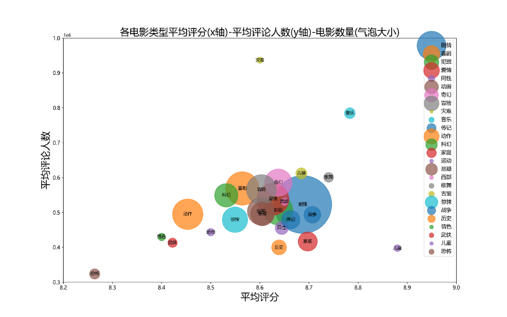
分析
通过气泡图可以发现,之前通过比例图发现占比高类型:剧情、喜剧、爱情、动作、冒险、犯罪等集中在平均评分8.4~8.8,平均评论人数300000-600000, 说明这些类型是热门题材,大众口味。但音乐、儿童题材平均评分更高,但影片数量少。恐怖题材的电影平均评分低,且平均评论人数少,推测原因可能是恐怖题材电影受众比较小,属于小众口味。而灾难题材电影评论人数多,但评分低,推测原因:电影中包含的特效镜头投入成本较高,造成拍片成本较高,所以评分会受电影特效观感的影响。
导演/演员-影片数分析
历史top500中导演人数与影片关系
# 历史top500中导演人数与影片关系
def director_work(self):
    """
         根据导演电影数生成矩形图
         :return:
         """

    to_drop = ['排名', '电影id', '名称', '演员', '年份', '国别', '类型', '语言', '评分', '评分人数', '五星占比', '四星占比', '三星占比', '二星占比',
               '一星占比', '短评数',
               '简介']
    res = self.newRows.drop(to_drop, axis=1)
    # 数据分割
    all_director_list = []
    for i in res.itertuples():
        #     print(i[1] + '\n')
        for j in i[1].split('/'):
            all_director_list.append(j)
    # 数据统计
    df = pd.DataFrame(all_director_list, columns=['导演'])
    res = df.groupby('导演')['导演'].count().sort_values(ascending=False)

    x=['[0,2)','[2,5)','[5,10)','[10,20)']
    y=[]
    x1=0
    x2=0
    x3=0
    x4=0

    for i in res.items():
        if i[1] in range(0,2):
            x1+=1
        if i[1] in range(2,5):
            x2+=1
        if i[1] in range(5, 10):
            x3 += 1
        if i[1] in range(10, 20):
            x4 += 1

    y.append(x1)
    y.append(x2)
    y.append(x3)
    y.append(x4)
    # 生成图表
    c = Bar()
    c.add_xaxis(x)
    c.add_yaxis("导演人数", y, color=Faker.rand_color())
    c.set_global_opts(
        title_opts=opts.TitleOpts(title="历史top500电影中导演人数-作品数"),
        yaxis_opts=opts.AxisOpts(name="导演人数"),
        xaxis_opts=opts.AxisOpts(name="作品数"),

    )
    # 生成html
    #c.render("历史top500电影中导演人数-作品数.html")
    return c
历史top500中演员人数与影片关系
# 历史top500中演员人数与影片关系
def star_work(self):
    """
         根据演员电影数生成柱状图
         :return:
         """
    to_drop = ['排名', '电影id', '名称', '导演', '年份', '国别', '类型', '语言', '评分', '评分人数', '五星占比', '四星占比', '三星占比', '二星占比',
               '一星占比', '短评数',
               '简介']
    res = self.newRows.drop(to_drop, axis=1)
    # 数据分割
    all_director_list = []
    for i in res.itertuples():
        #     print(i[1] + '\n')
        for j in i[1].split('/'):
            all_director_list.append(j)
    # 数据统计
    df = pd.DataFrame(all_director_list, columns=['演员'])
    res = df.groupby('演员')['演员'].count().sort_values(ascending=False)

    x=['[0,2)','[2,5)','[5,10)','[10,20)']
    y=[]
    x1=0
    x2=0
    x3=0
    x4=0

    for i in res.items():
        if i[1] in range(0,2):
            x1+=1
        if i[1] in range(2,5):
            x2+=1
        if i[1] in range(5, 10):
            x3 += 1
        if i[1] in range(10, 20):
            x4 += 1

    y.append(x1)
    y.append(x2)
    y.append(x3)
    y.append(x4)
    # 生成图表
    c = Bar()
    c.add_xaxis(x)
    c.add_yaxis("演员人数", y, color=Faker.rand_color())
    c.set_global_opts(
        title_opts=opts.TitleOpts(title="历史top500电影演员人数-作品数"),
        yaxis_opts=opts.AxisOpts(name="演员人数"),
        xaxis_opts=opts.AxisOpts(name="作品数"),

    )
    # 生成html
    #c.render("历史top500电影演员人数-作品数.html")
    return c
运行结果
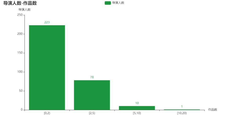
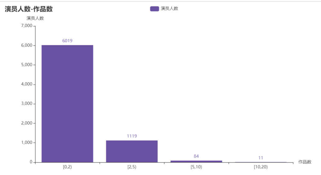
分析
对导演与演员进行分组,按照作品数量在[0,2), [2,5), [5,10), [10,20)进行分组统计作品上榜数量。从柱状图中发现导演与演员在历史上榜Top500中,在导演中共有312位导演上榜,有223位导演上榜1次;在演员中共有7233位演员参演,有6019位演员只参演过一次。多数人只参演过一部电影或只指导过一部电影,符合二八定律,即20%的人掌握80%的资源。
对2016-2021年top500与历史top500中重合电影进行分析
提取出优秀的电影
"""
按评分进行排序,取前10
按评论人数进行排序取前10
按短评数排序取前10
"""
def sort_Top10(self):
excel_path= '../kettle/common.xls'
rows = pd.read_excel(io=excel_path, sheet_name=0, header=0)
# 去空
rows.dropna(axis=0, how='any', inplace=True) # axis=0表示index行 "any"表示这一行或列中只要有元素缺失,就删除这一行或列
# 移除重复行
rows.drop_duplicates(subset=['电影id'], keep='first',inplace=True) # subset参数是一个列表,这个列表是需要你填进行相同数据判断的条件 keep=first时,保留相同数据的第一条。。inplace=True时,会对原数据进行修改。
# 按评分进行排序,取前10
b=rows.sort_values(by="评分" , ascending=False) #by 指定列 ascending
top10_score=b.head(10)
#print(top10_score)
# #按评分人数进行排序,取前10
b = rows.sort_values(by="评分人数", ascending=False) # by 指定列 ascending
top10_scorepeople = b.head(10)
#print(top10_scorepeople)
# #按短评数进行排序,取前10
b = rows.sort_values(by="短评数", ascending=False) # by 指定列 ascending
top10_commentpeople = b.head(10)
#print(top10_commentpeople)
#取交集
temp=pd.merge(top10_score, top10_scorepeople, how='inner')
result=pd.merge(top10_commentpeople, temp, how='inner')
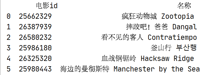
df = result[['电影id', '名称']]
print(df)
运行结果
对6部优秀电影进行情感分析
情感得分大于0.66为积极,小于0.33为消极
#情感分析
def make_sentiments_Pie(self):
    name_list=['疯狂动物城 Zootopia','摔跤吧!爸爸 Dangal','看不见的客人 Contratiempo','釜山行 부산행','血战钢锯岭 Hacksaw Ridge','海边的曼彻斯特 Manchester by the Sea']


    result_list = []
    for movie_name in name_list:
        filename = movie_name + '.csv'
        filpeath='../scrapy/comment/'+filename
        #csv_path='F:\python\豆瓣电影Top500\scrapy\comment\疯狂动物城 Zootopia.csv'
        df = pd.read_csv(filpeath)
        to_drop = ['用户', '是否看过', '评分', '评论时间', '有用数']
        df.drop(to_drop, axis=1, inplace=True)
        str = df.to_string(index=False, columns=['评论'], header=False)
        str = [i.strip() for i in str.split('\n')]

        result = {'positive': 0, 'negative': 0, 'neutral': 0}
        for i in str:
            s = SnowNLP(i)
            if (s.sentiments > 0.66):
                result['positive'] += 1
            elif (s.sentiments < 0.33):
                result['negative'] += 1
            else:
                result['neutral'] += 1
        result_list.append(result)
        # x=[]
        # for v in result.items():
        #     x.append(v)
        #
        # c.add("", x, center=["20%", "30%"], radius=[60, 80], )
    x_lists=[]
    for item in result_list:
        x=[]
        for v in item.items():
            x.append(v)
        x_lists.append(x)
    print("综合排名前6的电影情感得分")
    print(x_lists)

    # 生成图表
    c = Pie()

    c.set_global_opts(
        title_opts=opts.TitleOpts(title="排名前6电影评论的情感分析"),
        legend_opts=opts.LegendOpts(type_="scroll", pos_left="80%", orient="vertical"),
    )
    c.add('', x_lists[0], center=["20%", "30%"], radius=[30, 50], )
    c.add('', x_lists[1], center=["55%", "30%"], radius=[30, 50], )
    c.add('', x_lists[2], center=["20%", "60%"], radius=[30, 50], )
    c.add('', x_lists[3], center=["55%", "60%"], radius=[30, 50], )
    c.add('', x_lists[4], center=["20%", "90%"], radius=[30, 50], )
    c.add('', x_lists[5], center=["55%", "90%"], radius=[30, 50], )

    c.set_series_opts(label_opts=opts.LabelOpts(formatter="{b}: {c} ({d}%)"))
    # 生成html
    c.render("排名前6电影评论的情感分析.html")

    return c
运行结果
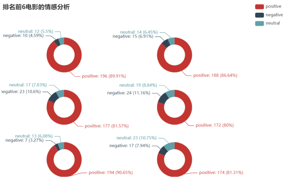
分析
可以发现选取的排名前6电影评论的情感得分为积极的占比超过80%,消极仅占11%以下。则这几部电影从评分、评论人数、短评数以及用户对其的评论角度进行选取的优质电影。
对6部优秀电影的评论进行词云分析
对6部优秀电影的评论进行词云分析
采用基于 TextRank 算法的关键词抽取,对每部电影的评论进行分词,去重停用词,统计词频,绘制词云图
plt.rcParams['font.sans-serif'] = ['SimHei']  # 用来正常显示中文标签
plt.rcParams['axes.unicode_minus'] = False  # 用来正常显示负号

class CommentAnalyse:

    def comment_cut_list(self,filename):
        """
        对一部影片的所有影评分词
        :param filename: 文件路径
        :return: segments -> list -> [{'word': '镜头', 'count': 1}, .....]
        """
        pd.set_option('max_colwidth', 500)  ##最大列字符数
        rows = pd.read_csv(filename, encoding='utf-8', dtype=str)
        to_drop = ['用户', '是否看过', '评分', '评论时间', '有用数']
        rows.drop(to_drop, axis=1, inplace=True)
        segments = []
        for index, row in rows.iterrows():
            content = row[0]
            # 第一个参数:待提取关键词的文本
            # 第二个参数:返回关键词的数量,重要性从高到低排序
            # 第三个参数:是否同时返回每个关键词的权重
            # 第四个参数:词性过滤,为空表示不过滤,若提供则仅返回符合词性要求的关键词
            # 同样是四个参数,但allowPOS默认为('ns', 'n', 'vn', 'v')
            # 即仅提取地名、名词、动名词、动词
            words = jieba.analyse.textrank(content, topK=20, withWeight=False, allowPOS=('ns', 'n', 'vn', 'v'))
            for word in words:
                segments.append({'word': word, 'count': 1})
        return segments


    def make_frequencies_df(self,segments):
        """
        传入分词list并返回词频统计后的 pandas.DataFrame对象
        :param segments: list -> [{'word': '镜头', 'count': 1}, .....]
        :return: pandas.DataFrame对象
        """
        # 加载停用词表
        stopwords = [line.strip() for line in open('../cn_stopwords.txt', encoding='UTF-8').readlines()]  # list类型
        # 去掉停用词的分词结果  list类型
        text_split_no = []
        for word in segments:
            if word.keys() not in stopwords:
                text_split_no.append(word)

        dfSg = pd.DataFrame(text_split_no)
        dfWord = dfSg.groupby('word')['count'].sum()    #根据word进行count的求和
        return dfWord

    def make_echarts(self,dfword, title):
        """
        利用pyecharts生成词云
        :param dfword: 词频统计后的 pandas.DataFrame对象
        :param title:
        :return:
        """

        htmlName = title + '.html'
        word_frequence = [(k, v) for k, v in dfword.items()]
        # print(word_frequence)
        wc = eWordCloud()
        wc.add(series_name="word", data_pair=word_frequence, word_size_range=[20, 100])
        wc.set_global_opts(title_opts=opts.TitleOpts(
                    title=title, pos_left="center", title_textstyle_opts=opts.TextStyleOpts(font_size=23)),
                    tooltip_opts=opts.TooltipOpts(is_show=True))
        wc.render(htmlName)
        return wc

    def make_wordcloud(self):
        name_list = ['疯狂动物城 Zootopia', '摔跤吧!爸爸 Dangal', '看不见的客人 Contratiempo', '釜山行 부산행', '血战钢锯岭 Hacksaw Ridge',
                     '海边的曼彻斯特 Manchester by the Sea']
        for movie_name in name_list:
            filename = movie_name + '.csv'
            filpeath = '../scrapy/comment/' + filename

        ###### pyecharts 生成词云 ######
            segments = self.comment_cut_list(filpeath)
            self.make_echarts(self.make_frequencies_df(segments), movie_name)
运行结果

分析
通过词云也可看出电影涉及的主题,主要人物。结合词云与情感分析可以看出这几部电影是备受好评的。且涉及的主题关于人性,成长,爱的话题,这些能引起人们的共鸣,引发人们的思考。
结论
- 欧美电影的仍占领市场主流,而中国电影也在崛起。2016-2021年美国电影发行量居世界第1,中国电影发行量居世界第4。但自2018年-2021年受疫情影响,美国电影发行量减少,而中国电影发行量增多。
- 2016-2021年中美电影发行量与评分比较中,可以发现中国电影的发行量在提升,且电影评分整体上也不错,但需要关注电影的质量,在2020年时电影评分出现比较大的分散。
- 最热门的三种类型电影为:剧情、喜剧、爱情。但热门题材的电影评分不是很高,平均评分8.4~8.8,但影片数量多。音乐、儿童题材平均评分更高,但影片数量少。恐怖题材的电影平均评分低,且平均评论人数少,推测原因可能是恐怖题材电影受众比较小,属于小众口味。
- 从评分,评论人数,短评数,用户评论角度选取出6部优秀电影:疯狂动物城,摔跤吧 爸爸,看不见的客人,釜山行,血战钢锯岭,海边的曼彻斯特。
参考
本项目用于大数据分析大作业,参考网上很多的分析以及代码,如下列出主要参考代码以及分析,如有侵权请联系我,会删除该文章
【1】 豆瓣电影数据分析 https://www.jianshu.com/p/74ab3c7f6ec4
【2】 kangvcar/MoviesAnalyse https://github.com/kangvcar/MoviesAnalyse
【3】气泡图参考
【4】可视化大屏参考
【5】情感分析参考
代码
代码存放在github上 代码链接
可搜wangyuna7723/MovieAnaylsis

 浙公网安备 33010602011771号