

yolov3源码分析keras(二)损失函数计算
一、前言
损失函数计算主要分析两部分一部分是yolo_head函数的分析另一部分为ignore_mask的生成的分析。
二、重要细节分析
2.1损失函数计算具体代码及部分分析
 1 def yolo_loss(args, anchors, num_classes, ignore_thresh=.5, print_loss=False):
 2     #args前三个元素为yolov3输出的预测值,后三个维度为保存的label 值
 3     '''Return yolo_loss tensor
 4
 5     Parameters
 6     ----------
 7     yolo_outputs: list of tensor, the output of yolo_body or tiny_yolo_body
 8     y_true: list of array, the output of preprocess_true_boxes
 9     anchors: array, shape=(N, 2), wh
10     num_classes: integer
11     ignore_thresh: float, the iou threshold whether to ignore object confidence loss
12
13     Returns
14     -------
15     loss: tensor, shape=(1,)
16
17     '''
18     num_layers = len(anchors)//3 # default setting
19     yolo_outputs = args[:num_layers]
20     y_true = args[num_layers:]
21     anchor_mask = [[6,7,8], [3,4,5], [0,1,2]] if num_layers==3 else [[3,4,5], [1,2,3]]
22     input_shape = K.cast(K.shape(yolo_outputs[0])[1:3] * 32, K.dtype(y_true[0])) #13*32=416  input_shape--->[416,416]
23     grid_shapes = [K.cast(K.shape(yolo_outputs[l])[1:3], K.dtype(y_true[0])) for l in range(num_layers)]#(13,13),(26,26),(52,52)
24     loss = 0
25     m = K.shape(yolo_outputs[0])[0] # batch size, tensor
26     mf = K.cast(m, K.dtype(yolo_outputs[0])) #mf为batchsize大小
27    #逐层计算损失
28     for l in range(num_layers):
29         object_mask = y_true[l][..., 4:5] # 取出置信度
30         true_class_probs = y_true[l][..., 5:]#取出类别信息
31         #yolo_head讲预测的偏移量转化为真实值,这里的真实值是用来计算iou,并不是来计算loss的,loss使用偏差来计算的
32         grid, raw_pred, pred_xy, pred_wh = yolo_head(yolo_outputs[l],
33              anchors[anchor_mask[l]], num_classes, input_shape, calc_loss=True) #anchor_mask[0]=[6,7,8]
34         pred_box = K.concatenate([pred_xy, pred_wh])                            #anchors[anchor_mask[l]]=array([[  116.,   90.],
35                                                                                                         # [  156., 198.],
36                                                                                                         # [  373., 326.]])
37         # Darknet raw box to calculate loss.
38         raw_true_xy = y_true[l][..., :2]*grid_shapes[l][::-1] - grid #根据公式将boxes中心点x,y的真实值转换为偏移量
39         raw_true_wh = K.log(y_true[l][..., 2:4] / anchors[anchor_mask[l]] * input_shape[::-1])#计算宽高的偏移量
40         raw_true_wh = K.switch(object_mask, raw_true_wh, K.zeros_like(raw_true_wh)) # avoid log(0)=-inf(后边有详细解释为什么这么操作)
41         box_loss_scale = 2 - y_true[l][...,2:3]*y_true[l][...,3:4]  #(2-box_ares)避免大框的误差对loss 比小框误差对loss影响大
42
43         # Find ignore mask, iterate over each of batch.
44         ignore_mask = tf.TensorArray(K.dtype(y_true[0]), size=1, dynamic_size=True)#定义一个size可变的张量来存储不含有目标的预测框的信息
45         object_mask_bool = K.cast(object_mask, 'bool')#映射成bool类型  1=true 0=false
46         def loop_body(b, ignore_mask):
47             true_box = tf.boolean_mask(y_true[l][b,...,0:4], object_mask_bool[b,...,0]) #剔除为0的行
48             iou = box_iou(pred_box[b], true_box) #一张图片预测出的所有boxes与所有的ground truth boxes计算iou 计算过程与生成label类似利用了广播特性这里不详细描述
49             best_iou = K.max(iou, axis=-1)#找出最大iou
50             ignore_mask = ignore_mask.write(b, K.cast(best_iou<ignore_thresh, K.dtype(true_box)))#当iou小于阈值时记录,即认为这个预测框不包含物体
51             return b+1, ignore_mask
52         _, ignore_mask = K.control_flow_ops.while_loop(lambda b,*args: b<m, loop_body, [0, ignore_mask])#传入loop_body函数初值为b=0,ignore_mask
53         ignore_mask = ignore_mask.stack()
54         ignore_mask = K.expand_dims(ignore_mask, -1) #扩展维度用来后续计算loss
55
56         # K.binary_crossentropy is helpful to avoid exp overflow.
57         #仅计算包含物体框的x,y,w,h的损失
58         xy_loss = object_mask * box_loss_scale * K.binary_crossentropy(raw_true_xy, raw_pred[...,0:2], from_logits=True)
59         wh_loss = object_mask * box_loss_scale * 0.5 * K.square(raw_true_wh-raw_pred[...,2:4])
60         #置信度损失既包含有物体的损失 也包含无物体的置信度损失
61         confidence_loss = object_mask * K.binary_crossentropy(object_mask, raw_pred[...,4:5], from_logits=True)+ \
62             (1-object_mask) * K.binary_crossentropy(object_mask, raw_pred[...,4:5], from_logits=True) * ignore_mask
63         #分类损失只计算包含物体的损失
64         class_loss = object_mask * K.binary_crossentropy(true_class_probs, raw_pred[...,5:], from_logits=True)
65         #取平均值
66         xy_loss = K.sum(xy_loss) / mf
67         wh_loss = K.sum(wh_loss) / mf
68         confidence_loss = K.sum(confidence_loss) / mf
69         class_loss = K.sum(class_loss) / mf
70         loss += xy_loss + wh_loss + confidence_loss + class_loss
71         if print_loss:
72             loss = tf.Print(loss, [loss, xy_loss, wh_loss, confidence_loss, class_loss, K.sum(ignore_mask)], message='loss: ')
73     return loss
2.2 yolo_head代码分析
yolo_head主要作用是将预测出的数据转换为真实值。代码如下:
 1 def yolo_head(feats, anchors, num_classes, input_shape, calc_loss=False):
 2     """Convert final layer features to bounding box parameters."""
 3     num_anchors = len(anchors) # num_anchors = 3
 4     # Reshape to batch, height, width, num_anchors, box_params.
 5     anchors_tensor = K.reshape(K.constant(anchors), [1, 1, 1, num_anchors, 2])#  [[[[[30.,   61.]
 6     grid_shape = K.shape(feats)[1:3] # height, width                                 [62.,   45.]
 7     grid_y = K.tile(K.reshape(K.arange(0, stop=grid_shape[0]), [-1, 1, 1, 1]),  #    [59.,  119.]]]]]
 8         [1, grid_shape[1], 1, 1])
 9     grid_x = K.tile(K.reshape(K.arange(0, stop=grid_shape[1]), [1, -1, 1, 1]),
10         [grid_shape[0], 1, 1, 1])
11     grid = K.concatenate([grid_x, grid_y])
12     grid = K.cast(grid, K.dtype(feats))
13
14     feats = K.reshape(
15         feats, [-1, grid_shape[0], grid_shape[1], num_anchors, num_classes + 5])#featuremap [N,13,13,3(20+5)]-->[N,13,13,3,(20+5)]
16
17     # Adjust preditions to each spatial grid point and anchor size.
18     box_xy = (K.sigmoid(feats[..., :2]) + grid) / K.cast(grid_shape[::-1], K.dtype(feats))#grid 为偏移 ,将x,y相对于featuremap尺寸进行了归一化
19     box_wh = K.exp(feats[..., 2:4]) * anchors_tensor / K.cast(input_shape[::-1], K.dtype(feats))#real box_wh
20     box_confidence = K.sigmoid(feats[..., 4:5])
21     box_class_probs = K.sigmoid(feats[..., 5:])
22     if calc_loss == True:
23         return grid, feats, box_xy, box_wh
24     return box_xy, box_wh, box_confidence, box_class_probs
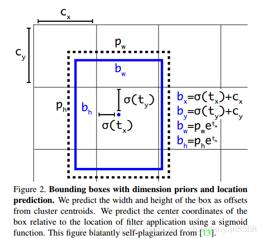
box真实值与预测值转换公式及示意图:
转换代码如下:
 box_xy = (K.sigmoid(feats[..., :2]) + grid) / K.cast(grid_shape[::-1], K.dtype(feats))#grid 为偏移
 box_wh = K.exp(feats[..., 2:4]) * anchors_tensor / K.cast(input_shape[::-1], K.dtype(feats))#real box_wh
对于初学者这个图也有一定的迷惑性质,可以把上图的每个网格想象成feature map上的一个点,则第一个像素对应的偏移为(0,0),第一行第二个偏移为(1,0)以此类推。图中标注的点偏移量为(1,1)。
yolo_head中转换为真实值时gride偏移相对于特征图尺寸做了归一化。
代码对于预测出的值进行了Sigmoid操作目的是为了让坐标值在0-1之间。
假设蓝色点为13*13的feature map 中的cell预测的中心点坐标为x,y,取sigmoid后其坐标为 (0.3, 0.5),则真实框在这个尺度上的中心点坐标值为(0.3+1, 0.5+1),映射到原图尺度为(1.3,1,5)*scale。
在这里scale=32。
其中grid为相对于feature map左上角的偏移量。以13*13的feature map为例来说明box 中心点x,y以及宽高w,h的计算过程。
K.arange(0, stop=grid_shape[0]) ---->[ 0, 1, 2, 3, 4, 5, 6, 7, 8, 9, 10, 11, 12]
K.reshape(K.arange(0, stop=grid_shape[0]), [-1, 1, 1, 1]) ----> -1表示为变化的维度,放在第一维度表示第一位维是变化的则 shape=[13,1,1,1] 一共包含13行值分别为0, 1, 2, 3, 4, 5, 6, 7, 8, 9, 10, 11, 12。
具体形式如下:[ [ [ [ 0 ] ] ]
..........
[ [ [12 ] ] ] ]
grid_y = K.tile(K.reshape(K.arange(0, stop=grid_shape[0]), [-1, 1, 1, 1]), [1, grid_shape[1], 1, 1]) ----> 表示在第二个维度重复13次 shape=[13,13,1,1]
具体形式如下:[ [ [ [ 0 ] ]
...........
[ [ 0 ] ] 重复13次
[ [ [ 1 ] ]
............
[ [ 1 ] ] 重复13次
.............
.............
[ [ [ 12 ] ]
...............
[ [12 ] ] ] ]
同理可得到grid_x的具体形式:[ [ [ [ 0 ] ] shape=[13,13,1,1]
[ [ 1 ] ]
............
[ [12 ] ] ]
.............
.............
[ [ [ [ 0 ] ] 蓝色部分共重复了13次
[ [ 1 ] ]
............
[ [ 12 ] ] ]
grid最终形式为 [ [ [ [ 0 0 ] ] shape=[13,13,1,2]
[ [ 1 0 ] ]
................
[ [12 1 ] ] ]
[ [ [ 0 1 ] ]
[ [ 1 1 ] ]
................
[ [12 1] ] ]
..................
..................
[ [ [ 0 12 ] ]
[ [ 1 12 ] ]
................
[ [12 12] ] ]
三、有关损失函数的一些注意事项
ps: 损失函数计算的为偏移量的损失,作者将真实的标签宽高转换为对应特征图尺寸上宽高的偏移量,然后与预测出的宽高偏移量计算误差。并不是将预测出的偏移转换为真实值和标签计算误差。 即计算的为偏移量的误差不是真实值之间的误差。同理中心点误差计算也是特征图上的中心点坐标。
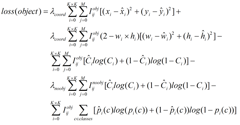
实际公式中xi,yi尖,为网络预测出的中心点值计算sigmoid之后的值。原版darknet计算中心点损失使用的是方差。keras作者使用的是交叉熵,这点有所不同。

 浙公网安备 33010602011771号