

Python_散点图与折线图绘制
在数据分析的过程中,经常需要将数据可视化,目前常使用的:散点图 折线图
需要import的外部包 一个是绘图 一个是字体导入
import matplotlib.pyplot as plt
from matplotlib.font_manager import FontProperties
在数据处理前需要获取数据,从TXT XML csv excel 等文本中获取需要的数据,保存到list
 1 def GetFeatureList(full_path_file):
 2     file_name = full_path_file.split('\\')[-1][0:4]
 3     # print(file_name)
 4     # print(full_name)
 5     K0_list = []
 6     Area_list = []
 7     all_lines = []
 8     f = open(full_path_file,'r')
 9     all_lines = f.readlines()
10     lines_num = len(all_lines)
11     # 数据清洗
12     if lines_num > 5000:
13         for i in range(3,lines_num-1):
14             temp_k0 = int(all_lines[i].split('\t')[1])
15             if temp_k0 == 0:
16                 K0_list.append(ComputK0(all_lines[i]))
17             else:
18                 K0_list.append(temp_k0)
19             Area_list.append(float(all_lines[i].split('\t')[15]))
20         # K0_Scatter(K0_list,Area_list,file_name)
21     else:
22         print('{} 该样本量少于5000'.format(file_name))
23     return K0_list, Area_list,file_name
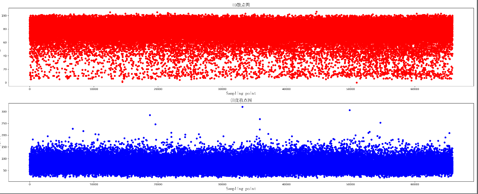
绘制两组数据的散点图,同时绘制两个散点图,上下分布在同一个图片中
 1 def K0_Scatter(K0_list, area_list, pic_name):
 2     plt.figure(figsize=(25, 10), dpi=300)
 3     # 导入中文字体,及字体大小
 4     zhfont = FontProperties(fname='C:/Windows/Fonts/simsun.ttc', size=16)
 5     ax = plt.subplot(211)
 6     # print(K0_list)
 7     ax.scatter(range(len(K0_list)), K0_list, c='r', marker='o')
 8     plt.title(u'散点图', fontproperties=zhfont)
 9     plt.xlabel('Sampling point', fontproperties=zhfont)
11     plt.ylabel('K0_value', fontproperties=zhfont)
12     ax = plt.subplot(212)
13     ax.scatter(range(len(area_list)), area_list, c='b', marker='o')
14     plt.xlabel('Sampling point', fontproperties=zhfont)
15     plt.ylabel(u'大小', fontproperties=zhfont)
16     plt.title(u'散点图', fontproperties=zhfont)
17     # imgname = 'E:\\' + pic_name + '.png'
18     # plt.savefig(imgname, bbox_inches = 'tight')
19     plt.show()
散点图显示
绘制一个折线图 每个数据增加标签
 1 def K0_Plot(X_label, Y_label, pic_name):
 2     plt.figure(figsize=(25, 10), dpi=300)
 3     # 导入中文字体,及字体大小
 4     zhfont = FontProperties(fname='C:/Windows/Fonts/simsun.ttc', size=16)
 5     ax = plt.subplot(111)
 6     # print(K0_list)
 7     ax.plot(X_label, Y_label, c='r', marker='o')
 8     plt.title(pic_name, fontproperties=zhfont)
 9     plt.xlabel('coal_name', fontproperties=zhfont)
10     plt.ylabel(pic_name, fontproperties=zhfont)
11     # ax.xaxis.grid(True, which='major')
12     ax.yaxis.grid(True, which='major')
13     for a, b in zip(X_label, Y_label):
14         str_label = a + str(b) + '%'
15         plt.text(a, b, str_label, ha='center', va='bottom', fontsize=10)
16     imgname = 'E:\\' + pic_name + '.png'
17     plt.savefig(imgname, bbox_inches = 'tight')
18     # plt.show()

绘制多条折线图
 1 def K0_MultPlot(dis_name, dis_lsit, pic_name):
 2     plt.figure(figsize=(80, 10), dpi=300)
 3     # 导入中文字体,及字体大小
 4     zhfont = FontProperties(fname='C:/Windows/Fonts/simsun.ttc', size=16)
 5     ax = plt.subplot(111)
 6     X_label = range(len(dis_lsit[1]))
 7     p1 = ax.plot(X_label, dis_lsit[1], c='r', marker='o',label='Euclidean Distance')
 8     p2 = ax.plot(X_label, dis_lsit[2], c='b', marker='o',label='Manhattan Distance')
 9     p3 = ax.plot(X_label, dis_lsit[4], c='y', marker='o',label='Chebyshev Distance')
10     p4 = ax.plot(X_label, dis_lsit[5], c='g', marker='o',label='weighted Minkowski Distance')
11     plt.legend()
12     plt.title(pic_name, fontproperties=zhfont)
13     plt.xlabel('coal_name', fontproperties=zhfont)
14     plt.ylabel(pic_name, fontproperties=zhfont)
15     # ax.xaxis.grid(True, which='major')
16     ax.yaxis.grid(True, which='major')
17     for a, b,c in zip(X_label, dis_lsit[5],dis_name):
18         str_label = c + '_'+ str(b)
19         plt.text(a, b, str_label, ha='center', va='bottom', fontsize=5)
20     imgname = 'E:\\' + pic_name + '.png'
21     plt.savefig(imgname,bbox_inches = 'tight')
22     # plt.show()

图形显示还有许多小技巧,使得可视化效果更好,比如坐标轴刻度的定制,网格化等,后续进行整理
posted on 2019-10-22 14:44 wangxiaobei2019 阅读(3614) 评论(0) 收藏 举报


 浙公网安备 33010602011771号