pytorch中文文档-torch.nn常用函数-待添加

https://pytorch.org/docs/stable/nn.html

1）卷积层

class torch.nn.Conv2d(in_channels, out_channels, kernel_size, stride=1, padding=0, dilation=1, groups=1, bias=True)

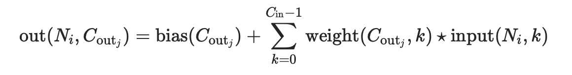
二维卷积层, 输入的尺度是(N, C_in,H,W)，输出尺度（N,C_out,H_out,W_out）的计算方式：

说明

stride: 控制相关系数的计算步长
dilation: 用于控制内核点之间的距离；可见pytorch的函数中的dilation参数的作用
groups: 控制输入和输出之间的连接：可见pytorch的函数中的group参数的作用

group=1，输出是所有的输入的卷积；
group=2，此时相当于有并排的两个卷积层，每个卷积层计算输入通道的一半，并且产生的输出是输出通道的一半，随后将这两个输出连接起来得到结果；
group=in_channels,每一个输入通道和它对应的卷积核进行卷积，该对应的卷积核大小为

参数kernel_size，stride,padding，dilation：

也可以是一个int的数据，此时卷积height和width值相同;
也可以是一个tuple数组，tuple的第一维度表示height的数值，tuple的第二维度表示width的数值，当是数组时，计算时height使用索引为0的值，width使用索引为1的值

Parameters：

in_channels(int) – 输入信号的通道
out_channels(int) – 卷积产生的通道
kerner_size(int or tuple) - 卷积核的尺寸
stride(int or tuple, optional) - 卷积步长，默认为1
padding(int or tuple, optional) - 输入的每一条边补充0的层数，默认为0
dilation(int or tuple, optional) – 卷积核元素之间的间距,默认为1
groups(int, optional) – 从输入通道到输出通道的阻塞连接数。默认为1
bias(bool, optional) - 如果bias=True，添加可学习的偏置到输出中

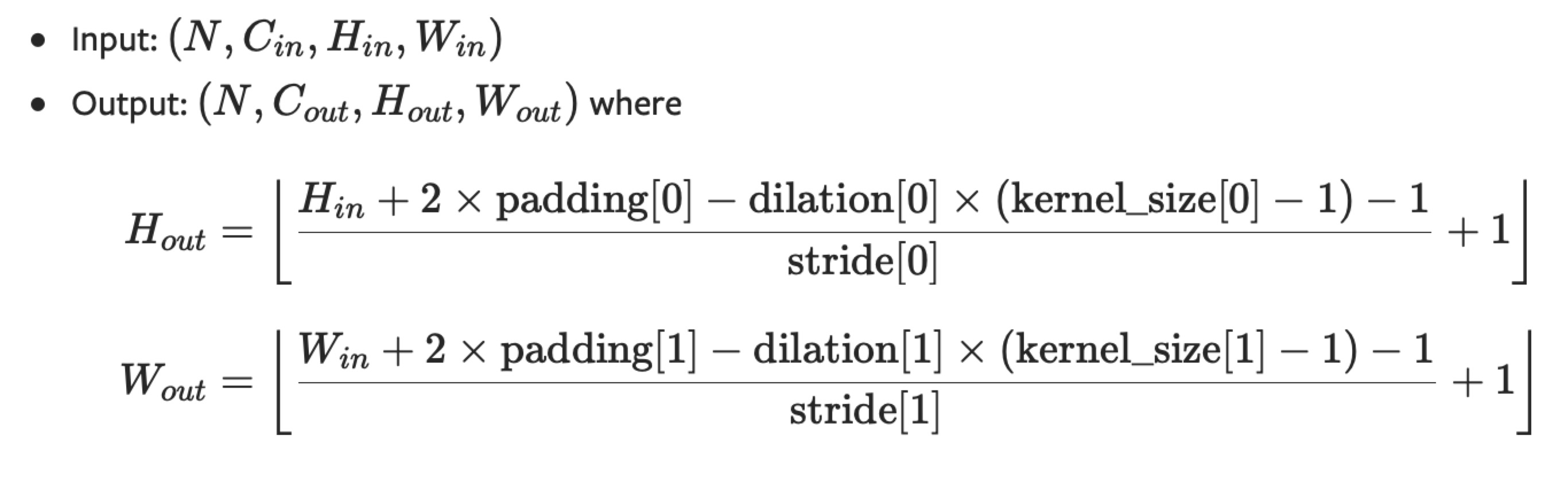
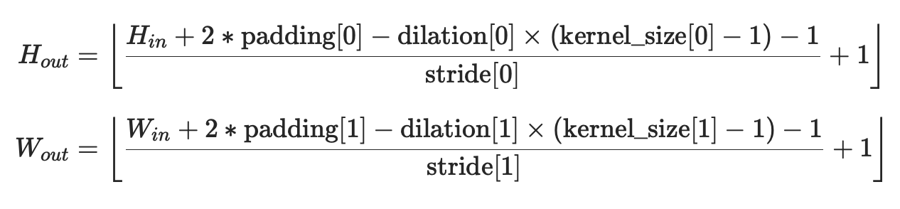
shape输出的height和width的计算式子:

变量:
weight(tensor) - 卷积的权重，大小是(out_channels, in_channels,kernel_size)
bias(tensor) - 卷积的偏置系数，大小是（out_channel）

class torch.nn.ConvTranspose2d(in_channels, out_channels, kernel_size, stride=1, padding=0, output_padding=0, groups=1, bias=True, dilation=1)

对由多个输入平面组成的输入图像应用二维转置卷积操作。

这个模块可以看作是Conv2d相对于其输入的梯度。它也被称为微步卷积(fractionally-strided convolutions)或解卷积(deconvolutions,尽管它不是一个实际的解卷积操作)。

说明

stride: 控制相关系数的计算步长
dilation: 用于控制内核点之间的距离
groups: 控制输入和输出之间的连接：

group=1，输出是所有的输入的卷积；
group=2，此时相当于有并排的两个卷积层，每个卷积层计算输入通道的一半，并且产生的输出是输出通道的一半，随后将这两个输出连接起来。

参数kernel_size，stride，padding，dilation数据类型：

可以是一个int类型的数据，此时卷积height和width值相同;
也可以是一个tuple数组（包含来两个int类型的数据），第一个int数据表示height的数值，第二个int类型的数据表示width的数值

注意
由于内核的大小，输入的最后的一些列的数据可能会丢失。因为输入和输出不是完全的互相关。因此，用户可以进行适当的填充（padding操作）。

padding参数有效地将 (kernel_size - 1)/2 数量的零添加到输入大小。这样设置这个参数是为了使Conv2d和ConvTranspose2d在初始化时具有相同的参数，而在输入和输出形状方面互为倒数。然而，当stride > 1时，Conv2d将多个输入形状映射到相同的输出形状。output_padding通过在一边有效地增加计算出的输出形状来解决这种模糊性。

注意，output_padding只用于查找输出形状，但实际上并不向输出添加零填充。

output_padding的作用：可见nn.ConvTranspose2d的参数output_padding的作用

在某些情况下，当使用CUDA后端与CuDNN，该操作可能选择一个不确定性算法，以提高性能。如果不希望出现这种情况，可以通过设置torch.backends.cudnn.deterministic = True使操作具有确定性(可能要付出性能代价)。有关背景资料，请参阅有关 Reproducibility的说明。

参数：

in_channels(int) – 输入信号的通道数
out_channels(int) – 卷积产生的通道数
kerner_size(int or tuple) - 卷积核的大小
stride(int or tuple,optional) - 卷积步长
padding(int or tuple, optional) - 输入的每一条边补充padding= kernel - 1 - padding,即(kernel_size - 1)/2个0的层数，所以补充完高宽都增加(kernel_size - 1)
output_padding(int or tuple, optional) - 在输出的每一个维度的一边补充0的层数，所以补充完高宽都增加padding，而不是2*padding，因为只补一边
dilation(int or tuple, optional) – 卷积核元素之间的间距
groups(int, optional) – 从输入通道到输出通道的阻塞连接数
bias(bool, optional) - 如果bias=True，添加偏置

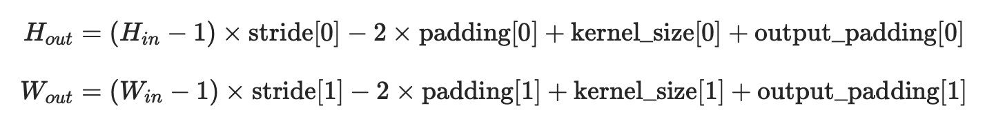
shape:
输入: (N,C_in,H_in，W_in)
输出: (N,C_out,H_out,W_out)

变量:
- weight(tensor) - 卷积的权重，大小是(in_channels, in_channels,kernel_size) ,从，中进行采样
- bias(tensor) - 卷积的偏置系数，大小是（out_channel） ,从，中进行采样

⚠️deconv只能做到还原输出大小到和 $X$

详细可见逆卷积的详细解释ConvTranspose2d（fractionally-strided convolutions)

举例：

import torch
from torch import nn
input = torch.randn(1,16,12,12)
downsample = nn.Conv2d(16,16,3,stride=2,padding=1)
upsample = nn.ConvTranspose2d(16,16,3,stride=2,padding=1)
h = downsample(input)
h.size()

torch.Size([1, 16, 6, 6])

output = upsample(h, output_size=input.size())
output.size()

torch.Size([1, 16, 12, 12])

如果没有指定：

output = upsample(h)
output.size()

返回将是：

torch.Size([1, 16, 12, 12])

使用output_padding也能解决这个问题：

upsample = nn.ConvTranspose2d(16,16,3,stride=2,padding=1,output_padding=1)

2）标准化层

class torch.nn.BatchNorm2d(num_features, eps=1e-05, momentum=0.1, affine=True)

对小批量(mini-batch)3d数据组成的4d输入进行批标准化(Batch Normalization)操作

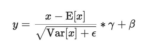
进行了两步操作：可见 Batch Normalization的解释 先对输入进行归一化，E(x)为计算的均值，Var(x)为计算的方差 然后对归一化的结果进行缩放和平移，设置affine=True，即意味着weight(γ)和bias(β)将被使用

在每一个小批量（mini-batch）数据中，计算输入各个维度的均值和标准差。γ与β是可学习的大小为C的参数向量（C为输入大小)。默认γ取值为U(0,1)， $β$ 设置为0

同样，默认情况下，在训练期间，该层将运行其计算的平均值和方差的估计值，然后在验证期间使用这些估计值（即训练求得的均值/方差）进行标准化。运行估计(running statistics)时保持默认momentum为0.1。

如果track_running_stats被设置为False，那么这个层就不会继续运行验证，并且在验证期间也会使用批处理统计信息。

⚠️这个momentum参数不同于优化器optimizer类中使用的momentum参数和momentum的传统概念。从数学上讲，这里运行统计数据的更新规则是 :

x是估计的数据
x_t是新的观察到的数据

x_new = (1-momentum) * x + momentum * x_t

因为批处理规范化是在C维(channel通道维度)上完成的，计算(N,H,W)片上的统计信息，所以通常将其称为空间批处理规范化。

参数：

num_features： C来自期待的输入大小(N,C,H,W)
eps： 即上面式子中分母的ε ，为保证数值稳定性（分母不能趋近或取0）,给分母加上的值。默认为1e-5。
momentum： 动态均值和动态方差所使用的动量。默认为0.1。
affine： 一个布尔值，当设为true，给该层添加可学习的仿射变换参数，即γ与β。
track_running_stats：一个布尔值，当设置为True时，该模块跟踪运行的平均值和方差，当设置为False时，该模块不跟踪此类统计数据，并且始终在train和eval模式中使用批处理统计数据。默认值:True

Shape：

输入：（N, C，H, W)

输出：（N, C, H, W）（输入输出相同）

举例：

当affine=True时

import torch
from torch import nn

m = nn.BatchNorm2d(2,affine=True)
print(m.weight)
print(m.bias)

input = torch.randn(1,2,3,4)
print(input)
output = m(input)
print(output)
print(output.size())

Parameter containing:
tensor([0.5247, 0.4397], requires_grad=True)
Parameter containing:
tensor([0., 0.], requires_grad=True)
tensor([[[[ 0.8316, -1.6250,  0.9072,  0.2746],
          [ 0.4579, -0.2228,  0.4685,  1.2020],
          [ 0.8648, -1.2116,  1.0224,  0.7295]],

         [[ 0.4387, -0.8889, -0.8999, -0.2775],
          [ 2.4837, -0.4111, -0.6032, -2.3912],
          [ 0.5622, -0.0770, -0.0107, -0.6245]]]])
tensor([[[[ 0.3205, -1.1840,  0.3668, -0.0206],
          [ 0.0916, -0.3252,  0.0982,  0.5474],
          [ 0.3409, -0.9308,  0.4373,  0.2580]],

         [[ 0.2664, -0.2666, -0.2710, -0.0211],
          [ 1.0874, -0.0747, -0.1518, -0.8697],
          [ 0.3160,  0.0594,  0.0860, -0.1604]]]],
       grad_fn=<NativeBatchNormBackward>)
torch.Size([1, 2, 3, 4])

当affine=False时

import torch
from torch import nn

m = nn.BatchNorm2d(2,affine=False)
print(m.weight)
print(m.bias)

input = torch.randn(1,2,3,4)
print(input)
output = m(input)
print(output)
print(output.size())

None
None
tensor([[[[-1.5365,  0.2642,  1.0482,  2.0938],
          [-0.0906,  1.8446,  0.7762,  1.2987],
          [-2.4138, -0.5368, -1.2173,  0.2574]],

         [[ 0.2518, -1.9633, -0.0487, -0.0317],
          [-0.9511,  0.2488,  0.3887,  1.4182],
          [-0.1422,  0.4096,  1.4740,  0.5241]]]])
tensor([[[[-1.2739,  0.0870,  0.6795,  1.4698],
          [-0.1811,  1.2814,  0.4740,  0.8689],
          [-1.9368, -0.5183, -1.0326,  0.0819]],

         [[ 0.1353, -2.3571, -0.2028, -0.1837],
          [-1.2182,  0.1320,  0.2894,  1.4478],
          [-0.3080,  0.3129,  1.5106,  0.4417]]]])
torch.Size([1, 2, 3, 4])

3）池化层

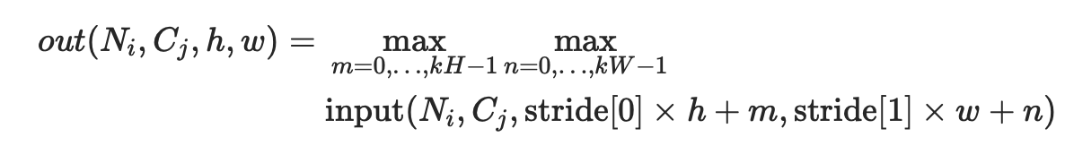
class torch.nn.MaxPool2d(kernel_size, stride=None, padding=0, dilation=1, return_indices=False, ceil_mode=False)

对于输入信号的输入通道，提供2维最大池化（max pooling）操作

如果输入的大小是(N,C,H,W)，那么输出的大小是(N,C,H_out,W_out)和池化窗口大小kernel_size(kH,kW)的关系是：

如果padding不是0，会在输入的每一边添加相应数目0
dilation用于控制内核点之间的距离

参数kernel_size，stride, padding，dilation数据类型：

可以是一个int类型的数据，此时卷积height和width值相同;
也可以是一个tuple数组（包含来两个int类型的数据），第一个int数据表示height的数值，tuple的第二个int类型的数据表示width的数值

参数：

kernel_size(int or tuple) - max pooling的窗口大小
stride(int or tuple, optional) - max pooling的窗口移动的步长。默认值是kernel_size
padding(int or tuple, optional) - 输入的每一条边补充0的层数
dilation(int or tuple, optional) – 一个控制窗口中元素步幅的参数
return_indices - 如果等于True，会返回输出最大值的序号，对于上采样操作torch.nn.MaxUnpool2d会有帮助
ceil_mode - 如果等于True，计算输出信号大小的时候，会使用向上取整ceil，代替默认的向下取整floor的操作

shape:
输入: (N,C,H_in,W_in)
输出: (N,C,H_out,W_out)

class torch.nn.AdaptiveAvgPool2d(output_size)

对输入信号，提供2维的自适应平均池化操作

Adaptive Pooling特殊性在于：

输出张量的大小都是给定的output_size。

例如输入张量大小为(1, 64, 8, 9)，设定输出大小为(5,7)，通过Adaptive Pooling层，可以得到大小为(1, 64, 5, 7)的张量

对于任何输入大小的输入，可以将输出尺寸指定为H*W，但是输入和输出特征的数目不会变化。

参数：

output_size: 输出信号的尺寸,可以用(H,W)表示H*W的输出，也可以使用单个数字H表示H*H大小的输出

举例：

input = torch.randn(1,64,8,9)
m = nn.AdaptiveAvgPool2d((5,7))
output = m(input)
output.shape

torch.Size([1, 64, 5, 7])

input = torch.randn(1,64,8,9)
m = nn.AdaptiveAvgPool2d(7)
output = m(input)
output.shape

torch.Size([1, 64, 7, 7])

4)非线形激活函数

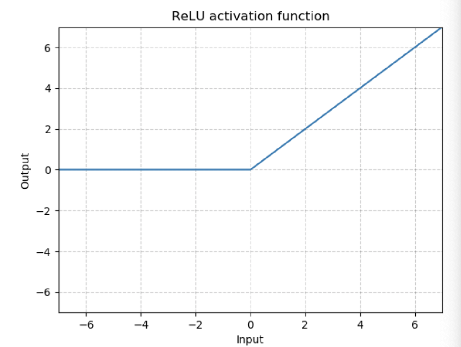
class torch.nn.ReLU(inplace=False)

对输入运用修正线性单元函数：

{ReLU}(x)= max(0, x)

图为：

参数： inplace-选择是否进行原位运算，即x= x+1

shape：

输入：(N,*), *代表任意数目附加维度
输出：(N,*)，与输入拥有同样的形状

举例：

import torch
from torch import nn
m = nn.ReLU()
input = torch.randn(2)
output = m(input)
input, output

(tensor([-0.0468,  0.2225]), tensor([0.0000, 0.2225]))

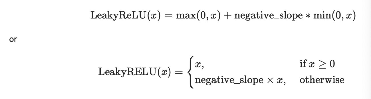
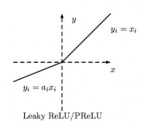
class torch.nn.LeakyReLU(negative_slope=0.01, inplace=False)

是ReLU的变形，Leaky ReLU是给所有负值赋予一个非零斜率

对输入的每一个元素运用：

参数：

negative_slope：控制负斜率的角度，默认等于0.01
inplace-选择是否进行原位运算，即x= x+1，默认为False

形状：

输入：(N,*), *代表任意数目附加维度
输出：(N,*)，与输入拥有同样的形状

图为：

举例：

m = nn.LeakyReLU(0.1)
input = torch.randn(2)
output = m(input)
input,output

(tensor([-1.3222,  0.8163]), tensor([-0.1322,  0.8163]))

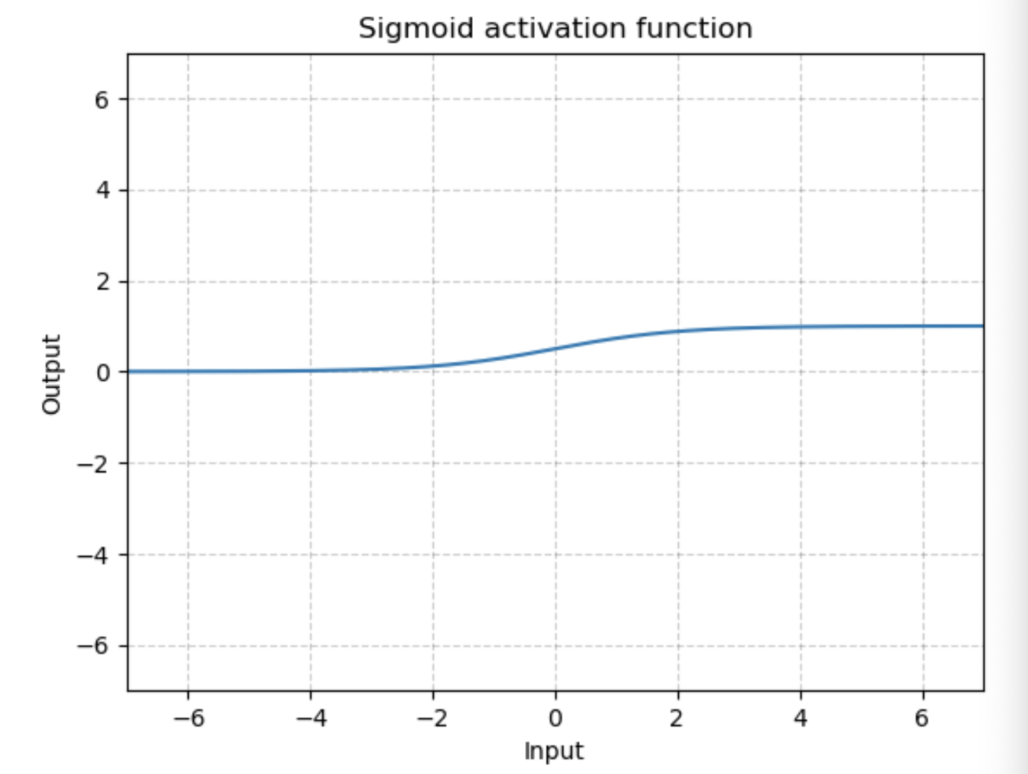
class torch.nn.Sigmoid

输出值的范围为[0,1]

提供元素方式函数：

形状：

输入：(N,*), *代表任意数目附加维度
输出：(N,*)，与输入拥有同样的形状

图为：

举例：

m = nn.Sigmoid()
input = torch.randn(2)
output = m(input)
input, output

(tensor([-0.8425,  0.7383]), tensor([0.3010, 0.6766]))

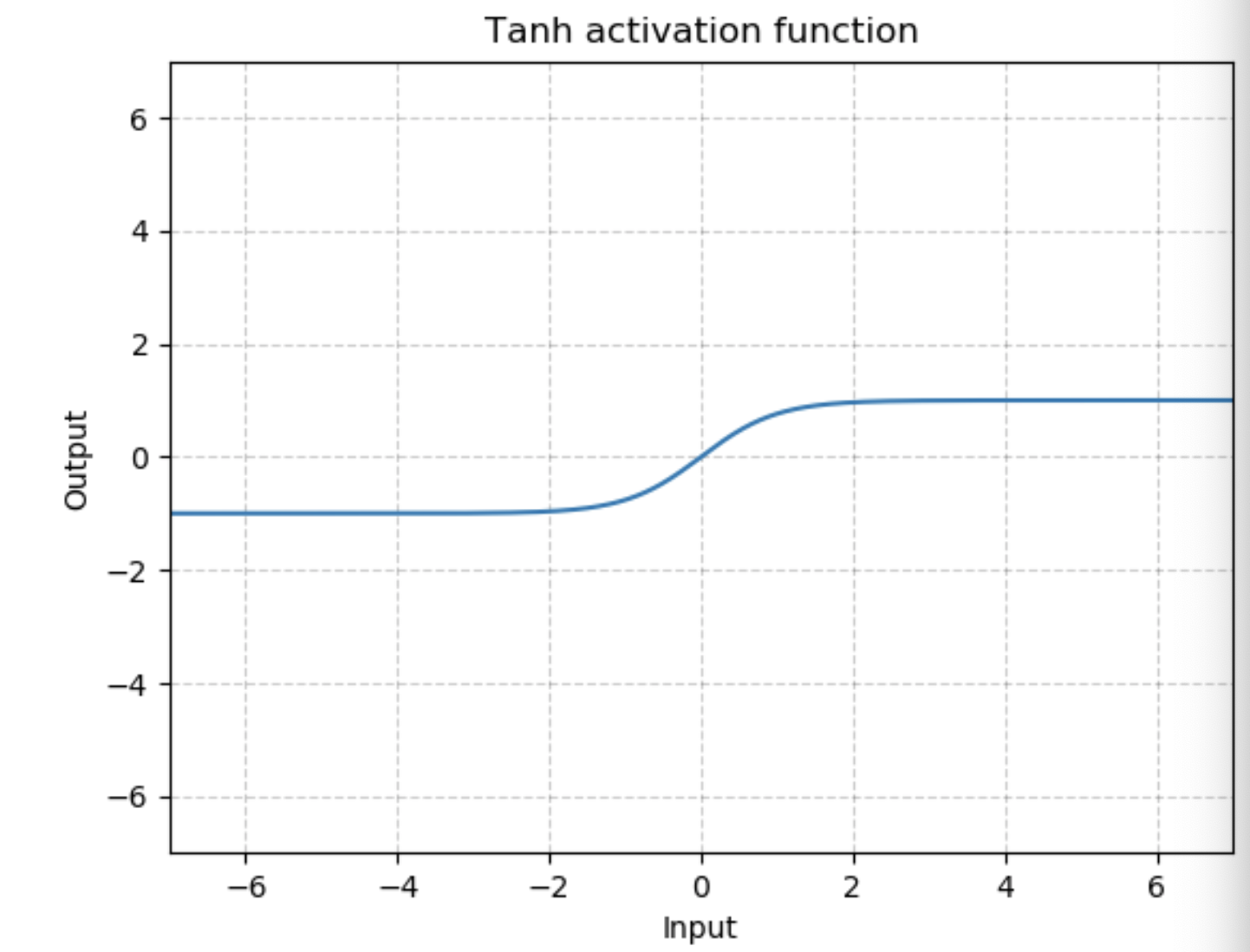
class torch.nn.Tanh

输出值的范围为[-1,1]

提供元素方式函数：

形状：

输入：(N,*), *代表任意数目附加维度
输出：(N,*)，与输入拥有同样的形状

图为：

举例：

m = nn.Tanh()
input = torch.randn(2)
output = m(input)
input, output

(tensor([-0.6246,  0.1523]), tensor([-0.5543,  0.1512]))

5）损失函数

class torch.nn.BCELoss(weight=None, size_average=True, reduce=None, reduction='mean')

计算 target 与 output 之间的二进制交叉熵。

损失函数能被描述为：

N是批处理大小。如果reduce=True,则：

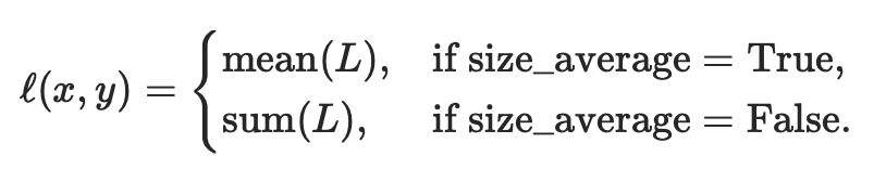
即默认情况下，loss会基于element求平均值，如果size_average=False的话，loss会被累加。

这是用来测量误差error的重建，例如一个自动编码器。注意 0<=target[i]<=1。

参数：

weight (Tensor,可选) – a manual rescaling weight given to the loss of each batch element. If given, has to be a Tensor of size “nbatch”.每批元素损失的手工重标权重。如果给定，则必须是一个大小为“nbatch”的张量。
size_average (bool, 可选) – 弃用(见reduction参数)。默认情况下，设置为True，即对批处理中的每个损失元素进行平均。注意，对于某些损失，每个样本有多个元素。如果字段size_average设置为False，则对每个小批的损失求和。当reduce为False时，该参数被忽略。默认值:True
reduce (bool,可选) – 弃用(见reduction参数)。默认情况下，设置为True，即根据size_average参数的值决定对每个小批的观察值是进行平均或求和。如果reduce为False，则返回每个批处理元素的损失，不进行平均和求和操作，即忽略size_average参数。默认值:True
reduction (string,可选) – 指定要应用于输出的reduction操作:' none ' | 'mean' | ' sum '。“none”:表示不进行任何reduction，“mean”:输出的和除以输出中的元素数，即求平均值，“sum”:输出求和。注意:size_average和reduce正在被弃用，与此同时，指定这两个arg中的任何一个都将覆盖reduction参数。默认值:“mean”

形状：

输入：(N,*), *代表任意数目附加维度
目标：(N,*)，与输入拥有同样的形状
输出:标量scalar，即输出一个值。如果reduce为False,即不进行任何处理，则(N,*)，形状与输入相同。

举例：

m = nn.Sigmoid()
loss = nn.BCELoss()
input = torch.randn(3,requires_grad=True)
target = torch.empty(3).random_(2)
output = loss(m(input), target)
output.backward()

input,target,output

(tensor([-0.8728,  0.3632, -0.0547], requires_grad=True),
 tensor([1., 0., 0.]),
 tensor(0.9264, grad_fn=<BinaryCrossEntropyBackward>))

input.grad

tensor([-0.2351,  0.1966,  0.1621])

posted @ 2019-04-28 15:58 慢行厚积阅读(26349) 评论(0) 编辑收藏举报

会员力量，点亮园子希望

刷新页面返回顶部

慢行厚积

pytorch中文文档-torch.nn常用函数-待添加

class torch.nn.Conv2d(in_channels, out_channels, kernel_size, stride=1, padding=0, dilation=1, groups=1, bias=True)

class torch.nn.ConvTranspose2d(in_channels, out_channels, kernel_size, stride=1, padding=0, output_padding=0, groups=1, bias=True, dilation=1)

class torch.nn.BatchNorm2d(num_features, eps=1e-05, momentum=0.1, affine=True)

class torch.nn.MaxPool2d(kernel_size, stride=None, padding=0, dilation=1, return_indices=False, ceil_mode=False)

class torch.nn.AdaptiveAvgPool2d(output_size)

class torch.nn.BCELoss(weight=None, size_average=True, reduce=None, reduction='mean')

公告