斐波那契数列的矩阵算法及 python 实现

目录

• 矩阵算法
• 通项公式
• 测试

import numpy as np
import matplotlib.pyplot as plt
from functools import reduce
from sympy import sqrt, simplify, fibonacci
import sympy

矩阵算法

斐波那契数的矩阵形式

\[\begin{align*} \begin{bmatrix} F_n\\ F_{n-1}\\ \end{bmatrix}&= \begin{bmatrix} 1&1\\ 1&0\\ \end{bmatrix}\cdot \begin{bmatrix} F_{n-1}\\ F_{n-2}\\ \end{bmatrix}\\ &=\begin{bmatrix} 1&1\\ 1&0\\ \end{bmatrix}^{n-1}\cdot \begin{bmatrix} F_1\\ F_0\\ \end{bmatrix}\\ \end{align*} \]

对于一个整数 \(n\)，可以写为二进制 \(n=\sum_{i=0}^{\lfloor\lg n\rfloor}2^in_i\)，其中 \(n_i\) 为 \(n\) 的二进制的各位数，\(n_i\in\lbrace0,1\rbrace\)。于是把上述公式写为

\[\begin{align*} \begin{bmatrix} F_n\\ F_{n-1}\\ \end{bmatrix}&\xlongequal{m\leftarrow n-1}\prod_{i=0}^{\lfloor\lg m\rfloor} \begin{bmatrix} 1&1\\ 1&0\\ \end{bmatrix}^{2^im_i}\cdot \begin{bmatrix} F_1\\ F_0\\ \end{bmatrix}\\ \end{align*} \]

可以先把 \(\begin{bmatrix}1&1\\1&0\\\end{bmatrix}^{2^i}\) 计算出来，再按照 \(m_i\) 相乘即可。

def fib1(n, dtype=sympy.Integer):
    if n == 0:
        return sympy.Integer(0)

    n -= 1
    bin_n = bin(n)[2:]    
    bool_n = list(map(bool, map(int, bin_n)))
    bool_n.reverse()

    m = [np.array([1, 1, 1, 0], dtype=dtype).reshape(2, 2)]
    for _ in range(len(bool_n) - 1):
        t = m[-1]
        m.append(np.matmul(t, t))

    needed = np.array(m)[bool_n]
    result = reduce(np.matmul, needed, np.eye(2, dtype=dtype))
    return result[0, 0]

采用 sympy.Integer 作为数据类型可以防止溢出。

分析时空复杂度：m 的长度为 \(\lfloor\lg(n-1)\rfloor+1\)，需要进行 \(\lfloor\lg(n-1)\rfloor\) 次 \(2\times2\) 的矩阵乘法；needed 的长度由 n-1 的二进制中的 1 的个数决定，但也不会超过 m 的长度。故时空复杂度约为 \(O(\lfloor\lg(n-1)\rfloor+1)=O(\lg n)\)。

但是考虑到使用大数字 sympy.Integer 进行乘法有与数字大小相关的开销。一般来说，这个开销约为 \(n^\alpha\)，其中 \(\alpha\) 约为 \(1.5\) 到 \(2\)，\(n\) 为相乘的两个数字的位数之和。

\(F_i = \frac{\phi^i-\hat\phi^i}{\sqrt5}\)，其中 \(\phi = \frac{1+\sqrt5}{2}, \hat\phi = \frac{1-\sqrt5}{2}\)，考虑到 \({\vert\hat\phi\vert\over\sqrt5}<\frac12\)，得到 \(F_i=\left\lfloor{\phi^i\over\sqrt5}+\frac12\right\rfloor\)，即斐波那契数以指数形式增长。

\[\begin{align*} m[i]&=\begin{bmatrix} F_{2^i+1}&F_{2^i}\\ F_{2^i}&F_{2^i-1} \end{bmatrix}\\ m[i]\cdot m[i]&=\begin{bmatrix} F_{2^i+1}^2+F_{2^i}^2&F_{2^i+1}F_{2^i}+F_{2^i}F_{2^i-1}\\ F_{2^i+1}F_{2^i}+F_{2^i}F_{2^i-1}&F_{2^i}^2+F_{2^i-1}^2\\ \end{bmatrix}\\ T(m[i]\cdot m[i])&\approx5cn^\alpha,\text{ where } n=2\left\lfloor\lg F_{2^i}\right\rfloor=2\lg\left\lfloor{\phi^{2^i}\over\sqrt5}+\frac12\right\rfloor\approx2^{i+1}\lg\phi-\lg5\\ &\approx5c(2^{i+1}\lg\phi)^\alpha\\ T(n)&=\sum_{i=0}^{\lfloor\lg(n-1)\rfloor-1}T(m[i]\cdot m[i])\\ &\approx5c\lg^\alpha\phi\sum_{i=0}^{\lfloor\lg(n-1)\rfloor-1}2^{\alpha(i+1)}\\ &=c'(2^{\alpha(\lfloor\lg(n-1)\rfloor+1)}-1)\\ &=\Theta(2^{\alpha\lg n})=\Theta(n^\alpha) \end{align*} \]

因此实际上的时间复杂度为 \(O(n^\alpha)\)，这个 \(\alpha\) 和选择的大数字乘法算法有关。

---

将数字转为二进制和计算矩阵的过程融合。

def fib2(n, dtype=sympy.Integer):
    m = np.array([1, 1, 1, 0], dtype=dtype).reshape(2, 2)
    result = np.eye(2, dtype=dtype)
    while n:
        if n & 1:
            result = result @ m
        m = m @ m
        n >>= 1
    return result[1, 0]

也可以不采用矩阵的形式。这表示我们要保存上述代码中 m 和 result 的值。

考虑矩阵

\[\begin{align*} \begin{bmatrix} 1&1\\ 1&0\\ \end{bmatrix}\cdot \begin{bmatrix} a+b&a\\ a&b \end{bmatrix}&=\begin{bmatrix} 2a+b&a+b\\ a+b&a \end{bmatrix}\\ &\xlongequal{a'\leftarrow a+b,b'\leftarrow a} \begin{bmatrix} a'+b'&a'\\ a'&b' \end{bmatrix} \end{align*} \]

所以形如 \(\begin{bmatrix}a+b&a\\a&b\end{bmatrix}\) 的对称矩阵与 \(\begin{bmatrix}1&1\\1&0\\\end{bmatrix}\) 相乘仍然是对称矩阵。

\[\begin{align*} \begin{bmatrix} p+q&p\\ p&q\\ \end{bmatrix}\cdot \begin{bmatrix} p+q&p\\ p&q\\ \end{bmatrix}&=\begin{bmatrix} (p+q)^2+p^2&p^2+2pq\\ p^2+2pq&p^2+q^2 \end{bmatrix}\\ &\xlongequal{p'\leftarrow p^2+2pq,q'\leftarrow p^2+q^2} \begin{bmatrix} p'+q'&p'\\ p'&q' \end{bmatrix}\\ \begin{bmatrix} p+q&p\\ p&q\\ \end{bmatrix}\cdot \begin{bmatrix} a+b&a\\ a&b\\ \end{bmatrix}&=\begin{bmatrix} (p+q)(a+b)+ap&a(p+q)+bp\\ a(p+q)+bp&ap+bq \end{bmatrix}\\ &\xlongequal{a'\leftarrow a(p+q)+bp,b'\leftarrow ap+bq} \begin{bmatrix} a'+b'&a'\\ a'&b' \end{bmatrix} \end{align*} \]

因此由于矩阵的特殊性，对于 m 我们只需要保存两个变量 \(p,q\)，对于 result 也只需要保存两个变量 \(a,b\)。

初始时有 \(m=\begin{bmatrix}1&1\\1&0\\\end{bmatrix},result=\begin{bmatrix}1&0\\0&1\\\end{bmatrix}\)，所以初始化 \(a=0,b=1,p=1,q=0\)。

def fib3(n, dtype=sympy.Integer):
    one, zero = dtype(1), dtype(0)
    a, b, p, q =  zero, one, one, zero
    while n:
        if n & 1:
            ap = a * p
            a, b = ap + a*q + b*p, ap + b*q
        pp = p * p
        p, q = pp + 2*p*q, pp + q*q
        n >>= 1
    return a

---

通项公式

在我前面的文章算法导论 Introduction to Algorithms #算法基础中，也证明了 \(F_i = \frac{\phi^i-\hat\phi^i}{\sqrt5}\)，其中 \(\phi = \frac{1+\sqrt5}{2}, \hat\phi = \frac{1-\sqrt5}{2}\)。

def fib4(n):
    p = (1 + sqrt(5)) / 2
    q = (1 - sqrt(5)) / 2
    return simplify((p ** n - q ** n) / sqrt(5))

---

测试

尝试用 Jupyter Notebook 测试算法速度，其中 fibonacci() 为 sympy 自带的斐波那契函数，三者返回的结果都为 sympy.Integer。

n = list(range(8, 17))
f = [fib1, fib2, fib3, fib4, fibonacci]
t = [[] for _ in range(len(f))]

for i in n:
    times = 2 ** i
    for j in range(len(f)):
        a = %timeit -o f[j](times)
        t[j].append(a.average)

plt.figure(figsize=(12, 8))
for j in range(len(f)):
    plt.subplot(2, 3, j + 1)
    plt.plot(n, t[j], label=f[j].__name__)
    plt.legend()
plt.show()

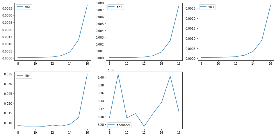
虽然用公式 \(F_i = \frac{\phi^i-\hat\phi^i}{\sqrt5}\) 看上去简洁明了，但是由于求指数没有经过优化、比较花时间。

sympy 内置的 fibonacci() 实际上调用了 mpmath.libmp 库中的 ifib() 函数。在计算的时候使用的数据类型不是 sympy.Integer，而是其他更接近底层的数据类型，所以速度会更快。

使用 np.log2() 取 \(\lg\)，再使用 np.polyfit(n, t, 1) 进行直线拟合，得到曲线和系数

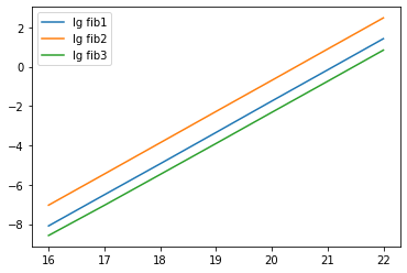
得到 \(\alpha\approx1.58\)，符合前面的时间复杂度的计算。

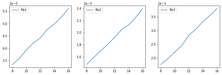
如果使用 np.int32 作为数据类型，那么就没有大数字的开销了，曲线为对数。