Plotdf from maxima

http://maxima.sourceforge.net/docs/manual/de/maxima_66.html#SEC354

Examples:

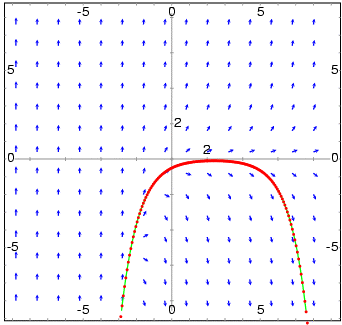
• To show the direction field of the differential equation y' = exp(-x) + y and the solution that goes through (2, -0.1):
• (%i1) plotdf(exp(-x)+y,[trajectory_at,2,-0.1])$

  

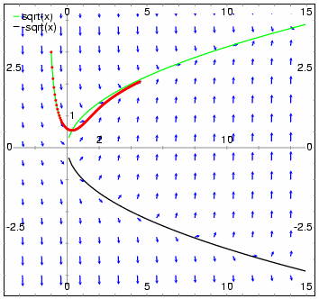
• To obtain the direction field for the equation diff(y,x) = x - y^2 and the solution with initial condition y(-1) = 3, we can use the command:
• (%i1) plotdf(x-y^2,[xfun,"sqrt(x);-sqrt(x)"],
• [trajectory_at,-1,3], [direction,forward],
• [y,-5,5], [x,-4,16])$

  The graph also shows the function y = sqrt(x).

  

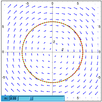
• The following example shows the direction field of a harmonic oscillator, defined by the two equations dz/dt = v and dv/dt = -k*z/m, and the integral curve through (z,v) = (6,0), with a slider that will allow you to change the value of m interactively (k is fixed at 2):
• (%i1) plotdf([v,-k*z/m], [z,v], [parameters,"m=2,k=2"],
• [sliders,"m=1:5"], [trajectory_at,6,0])$

  

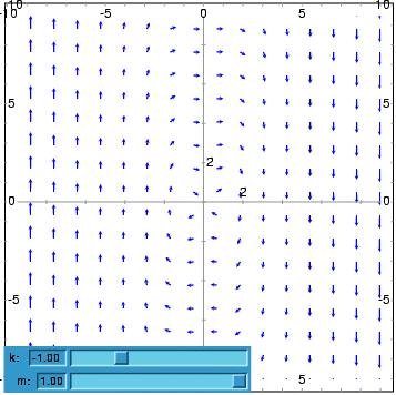
• To plot the direction field of the Duffing equation, m*x"+c*x'+k*x+b*x^3 = 0, we introduce the variable y=x' and use:
• (%i1) plotdf([y,-(k*x + c*y + b*x^3)/m],
• [parameters,"k=-1,m=1.0,c=0,b=1"],
• [sliders,"k=-2:2,m=-1:1"],[tstep,0.1])$

  

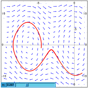
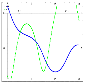
• The direction field for a damped pendulum, including the solution for the given initial conditions, with a slider that can be used to change the value of the mass m, and with a plot of the two state variables as a function of time:
• (%i1) plotdf([w,-g*sin(a)/l - b*w/m/l], [a,w],
• [parameters,"g=9.8,l=0.5,m=0.3,b=0.05"],
• [trajectory_at,1.05,-9],[tstep,0.01],
• [a,-10,2], [w,-14,14], [direction,forward],
• [nsteps,300], [sliders,"m=0.1:1"], [versus_t,1])$