Linear and Rotational Dynamics 学习

Linear and Rotational Dynamics

• " Cause" ot motion,force(12.1)
• particularly important and simple types of forces (12.2)
• momentum and relationship between force and momentum(12.3)
• collisions and impulse (12.4)
• rotation of objects and the angular analogs of the linear concepts(12.5)
• simulations(12.6)

12.1

Newton’s Second Law:

\[f = ma \]

The basic procedure is as follows,starting with a representation of the object.

1. Draw and label all the forces acting on it.
2. Sum up those forces (using vector addition) to compute the net force.
3. Use Newton’s second law (Equation (12.2)) to compute the acceleration of the object.
4. Integrate the acceleration to determine the motion of the object.

12.2

• Gravitational Force

  • Law of Universal Gravitation:
    $ f = G\frac{m_{1}m_{2}}{d^2} $

• Frictional Forces

  • static friction
    prevents bowls of petunias sitting on slightly inclined tables from sliding off.

    Static friction : $ f_s = u_sn $;
    the u is known as the coefficient of static friction and the n is the magnitude of the normal force.

  • kinetic friction

    kinetic friction : \(f_k = u_kn\); kinetic friction is usually less than the coefficient of static
    friction.

• Spring Forces

  rest length

  When the spring is at equilibrium with
  no external forces on it, it has a natural length, called the rest length.\(l_{rest}\) denote the rest length.
  Hooke’s law:
  The force law for springs is known as Hooke’s law, and it basically says
  that the magnitude of the restorative force is proportional to the difference
  from the current length and the rest length.If we let \(l\) be the current length of the spring and \(l_{rest}\) denote the rest length, then the magnitude of the restoring force fr is
  calculated:

\[f_{r} = k(l_{rest}-l) \]

Simple Harmonic Motion

\[x(t) = Acos(\omega t+ \theta_{0}) \]

\[\dot{x}(t) = -A\omega sin(\omega t+ \theta_{0}) \]

\[\ddot{x}(t) = -A\omega^{2} cos(\omega t+ \theta_{0}) \]

write the equation of motion directly in terms of frequency

\[x(t) = Acos(2\pi Ft + \theta_{0}) \]

damping force

\[f_{d} = -c x\dot{} \]

Combining the restorative and damping forces,the net force can be written as:
\(f_{net} = f_{r} + f_{d} = -kx - cx\dot{}\)

Applying Newton's second law,we have:$$ \ddot{x} = \frac{f_{net}}{m} = -\frac{k}{m}x - \frac{c}{m} \dot{x} \quad\quad\quad\quad\quad (12.11)$$

damping ratio
Now，The first quantity \(w_{0}\) is the undamped angular frequency,the second quantity is \(\zeta\),is damping ratio. The damping ratio is related to the damping coefficient, mass, and undamped angular frequency by the formula:

\[\zeta = \frac{c}{2\sqrt{mk}} = \frac{c}{2m\omega_{0}} \]

Substituting the undamped frequency \(\omega_{0}\) and damping ratio \(\zeta\) into Equation (12.11), we have

\[\ddot{x} = -\omega_{0}^2 - 2\zeta\omega_{0}\dot{x} \]

开始解这个方程:
There are three distinct cases: underdamping,critical damping,and overdamping.
Where $ 0 \leq \zeta < 1 $ is underdamped.This motion is:

\[x(t) = (k_{1}cow(\omega_{d}t) + k_{2}sin(\omega_{d}t))e^{-\zeta\omega_{0}t} \]

where \(\omega_{d}\)is the actual frequency of the damped oscillation and is related
to the undamped frequency \(\omega_{0}\) by $\omega_{d} = \omega_{0} \sqrt{1-\zeta^2} $
The constants \(k_{1}\) and \(k_{2}\) are determined by the initial position and velocity:
$k_{1} = x(0)， k_{2}=\frac{\zeta\omega_{0}x(0) + \dot{x}(0)}{w_{d}} $
The motion will continue to oscillate indefinitely with an amplitude that decays exponentially over time. (指数衰减)

Using\(\zeta == 0\),undamped oscillation.

when \(\zeta == 1\) critical damping: the frequency completely vanishes.The system
no longer oscillates, but instead decays exponentially. The kinematic
equation in this situation is:
\(x(t) = (k_{1} + k_{2}t)e^{-\omega_{0}t}\) where \(k_{1}\) and \(k_{2}\) are again determined by the initial conditions:
$$ k_{1} = x(0), \qquad k_{2} = \omega_{0}x(0) + \dot{x}(0) $$

Critical damping is just the right amount such that the system decays
as quickly as possible without oscillation. If the damping is decreased, the
system is underdamped, as previously described, and will oscillate. If the
damping is increased, the system is overdamped; it will not oscillate, and the
rate of decay will be slower than the rate at critical damping. Figure 12.6
shows how the damping value affects the behavior of a system.

12.3 Momentum

Momentum as Product of Mass and Velocity:

\[P = mv \]

Force as the Derivative of Momentum

\[\frac{d}{dt}P(t) = f(t) \]

Force as the Derivative of Momentum (动量守恒)

12.4 Impulsive Forces and Collisions

\[p_{1} = m_{1}v_{1} , \quad p_{2} = m_{2}v_{2} , \qquad p = p_{1} + p_{2} = m_{1}v_{1} +m_{2}v_{2} \]

\[p_{1}' = m_{1}v_{1}' , \quad p_{2}' = m_{2}v_{2}' , \qquad p = p_{1}' + p_{2}' = m_{1}v_{1}' +m_{2}v_{2}' \]

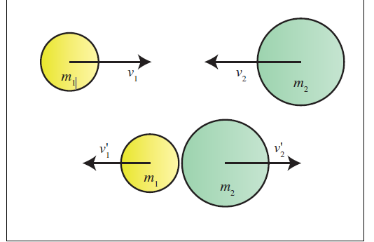
A likely scenario is for them to bounce off of each
other, changing the signs of both v1 and v2. Or they may stick together.
The former is known as an elastic collision and the latter an inelastic collision.

General Collision Response

Dealing with collisions is typically a two step process. First, we must detect that a collision (collision detection) has occurred, meaning the objects are already penetrating, or that a collision is about to occur in this time step. The second step is to take measures to resolve(collision response) or prevent the collision.

Of course, a collision doesn’t necessarily happen at a single point. Often an edge of one object may touch a surface of another, or perhaps entire surfaces are in contact. At the time of this writing, most real-time collision detection systems do not return collisions in such a descriptive manner, nor are collision response systems really capable of making use of that extra information. The closest we get is for the detection system to locate several points of contact (or penetration) and then to process that list in some way (for example, by finding their convex hull or looking for an average surface normal).

How do we determine the resulting velocities for the collision response?
Two guiding principle:

• That is, we will not be calculating a force, but rather an impulse, which will result in an instantaneous change in momentum of the objects.
• whatever (impulsive) force is applied to one object, the opposite force must be applied to the other object. The conservation of momentum law essentially says the same thing.

Thus, to resolve a collision between two objects, the game plan is to compute an impulse with the proper magnitude and apply that impulse to both objects, but in opposite directions.An impulse is a vector quantity, and so we need to know its magnitude and direction.The direction is surface normal provided by the collision detection system.
Our task is to determine the proper magnitude of an impulse that will be directed along the surface normal and will resolve (or prevent) the penetration.

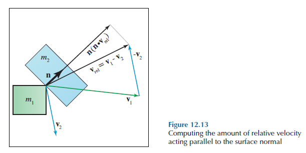
Newton’s collision law（not the only one） is A simple and popular collision law. This law introduces the coefficient of restitution, denoted \(e\), which is a fractional number that relates the magnitude of the relative velocity along the surface normal after the collision with the same value measured just before the collision. Let’s denote the magnitude of the collision response impulse as \(k\) . The first mass, \(m_{1}\), will receive the (vector) impulse \(−kn\), while \(m_{2}\) undergoes the opposite change in momentum of \(kn\).An impulse is an instantaneous change of momentum,

so the post-collision momentum of the first object is \(P'_{1} = P_{1} −kn\). Dividing by the mass and remembering \(P = mv\), we express the post-collision velocities as

\[v_{1}' = v_{1} - \frac{kn}{m_{1}} \qquad v_{2}' = v_{2} + \frac{kn}{m_{2}} \]

The post-collision relative velocity is simply their difference, \(v'_{rel} = v'_{1} −v'_{2}.\).
现在开始解决\(k\)了哦:

\[k = \frac{(e + 1)v_{rel}\cdot n}{(1/m_{1} + 1/m_{2})n\cdot n} \qquad \qquad \qquad (12.23) \]