MATLAB Gallery

组内用的比较专业的出图MATLAB代码：

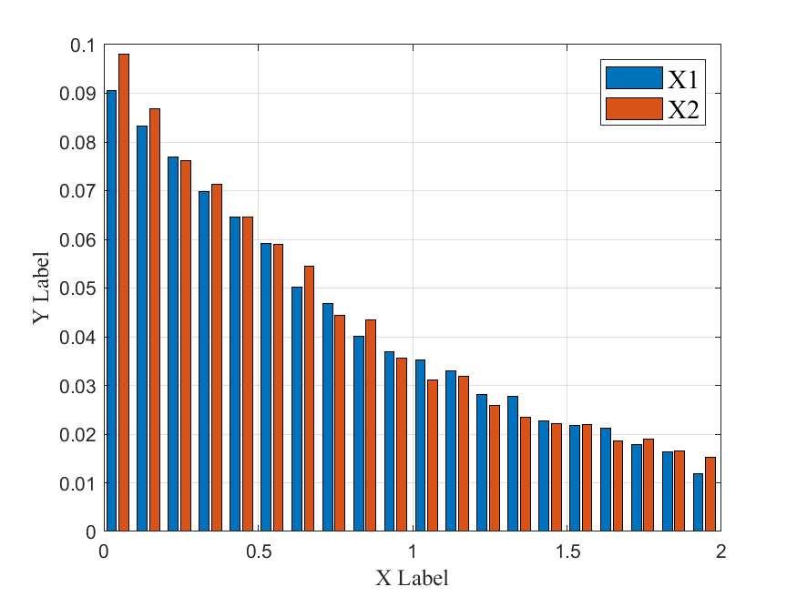
rng(10);
N = 10000;
X1 = exprnd(1, 1, N);
X2 = exprnd(1, 1, N);

ft = 'times new roman';
f1 = figure(1);
x = 0:0.1:2;

[N1,edges1] = histcounts(X1, x);
[N2,edges2] = histcounts(X2, x);
h1 = N1 ./ length(X1);
h2 = N2 ./ length(X2);

w = 0.05;
w2 = 0.03;

x = x + (x(2) - x(1)) / 2;
x = x(1:end - 1);

bar(x - w/2, h1, 0.32);
hold on
bar(x + w2/2, h2, 0.32);
grid on
xlim([0,2])

xlabel('X Label', 'FontSize',12, 'FontName', ft)
ylabel('Y Label', 'FontSize',12,'FontName', ft)

legend({'X1', 'X2'}, 'FontSize',14,...
     'FontName', ft);

saveas(f1,'results.png')
saveas(f1,'results','epsc')

addpath('plottools')  % 需要这部分向我要一下。
f1 = figure(1);
rng(10)
ft = 'times new roman';
cm = colororder; % or replace with the desired colormap

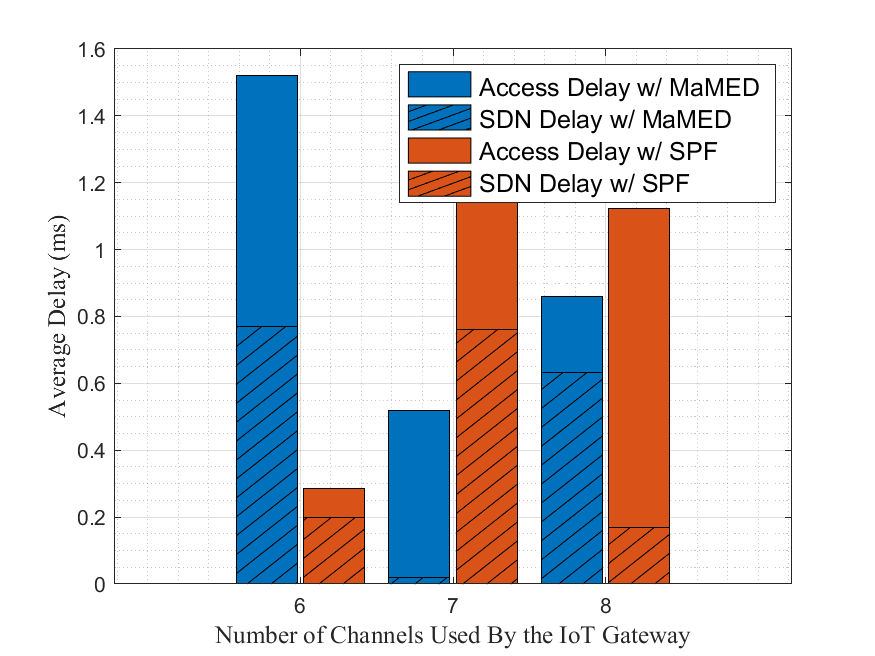
x = 6:8;

y1 = rand(3, 2);
y2 = rand(3, 2);

barflow = bar(x - 0.22, y1, 0.4, 'stacked');
barflow(1).FaceColor = cm(1,:);
hatchfill2(barflow(1),'single','HatchAngle',45,'hatchcolor','black');
barflow(2).FaceColor = cm(1,:);

hold on
barospf = bar(x + 0.22, y2, 0.4, 'stacked');
barospf(1).FaceColor = cm(2,:);
barospf(2).FaceColor = cm(2,:);
hatchfill2(barospf(1),'single','HatchAngle',45,'hatchcolor','black');

xlim([5.5 8.5])
grid minor

xticks(6:8)
xticklabels({'6','7','8'})

bars = [barflow, barospf];
legendData = {'Access Delay w/ MaMED','SDN Delay w/ MaMED',...
    'Access Delay w/ SPF', 'SDN Delay w/ SPF'};

[legend_h, object_h, plot_h, text_str] = ...
    legendflex(bars, legendData, 'Padding', ...
    [2, 2, 10], 'FontSize', 12);

hatchfill2(object_h(6), 'single', 'HatchAngle', 45, 'HatchDensity', 80/4, 'HatchColor', 'black');
hatchfill2(object_h(8), 'single', 'HatchAngle', 45, 'HatchDensity', 80/4, 'HatchColor', 'black');

grid on
xlabel('Number of Channels Used By the IoT Gateway','FontSize', 12, 'FontName', ft)
ylabel('Average Delay (ms)','FontName', ft, 'FontSize', 12)

saveas(f1,'delay_comparison.png')
saveas(f1,'delay_comparison','epsc')

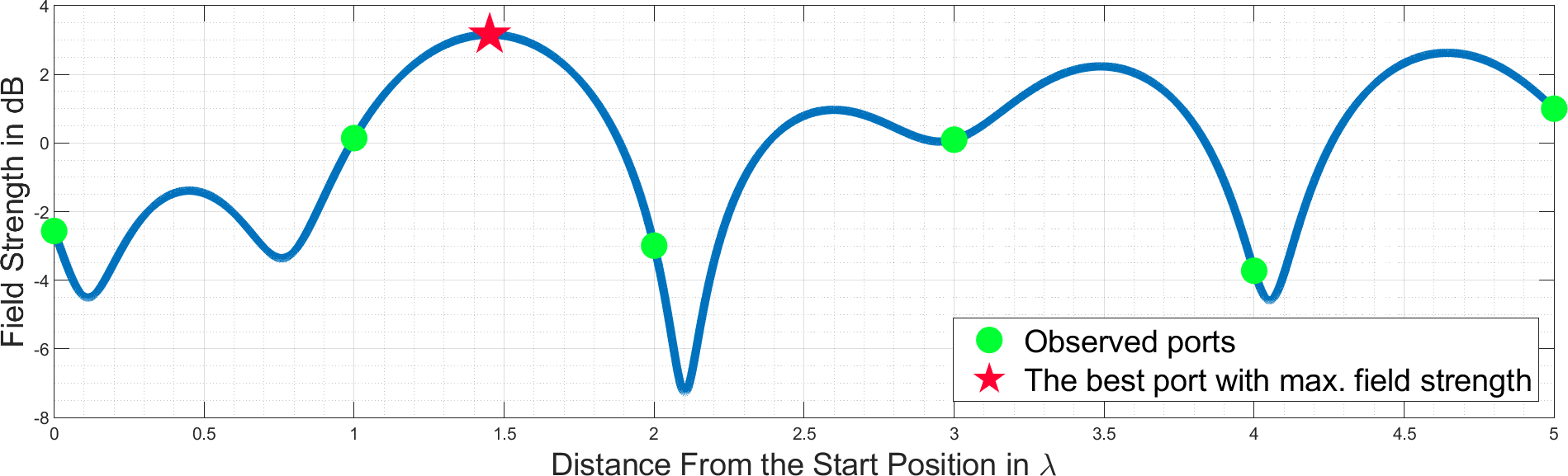
rng(13)
K = 1;
Np = 2;
W = 5;
N = 30;
Omega = 1;
alpha = rand * 2 * pi;
% Scattered components
a = (randn(1, Np) + 1i * randn(1, Np))/sqrt(2) * sqrt(Omega / (K + 1) / Np);
theta0 = rand * 2 * pi;
phi0 = rand * 2 * pi;
theta = rand(1, Np) * 2 * pi;
phi = rand(1, Np) * 2 * pi;
k = 0:0.01:N;
sampled = linspace(1, length(k), 6);

g = sqrt(K * Omega / (K + 1)) * exp(1i * alpha) * exp(-1i * 2 * pi * (k - 1) ...
    * W * sin(theta0) * cos(phi0) / (N - 1))+ a * exp(-1i * 2 * pi * W * ...
    (sin(theta) .* cos(phi))' .*(k - 1)/(N -1));

g = 10 * log10(abs(g));

[M, loc] = max(g);

f1 = figure(1);
f1.Position = [100 100 1500 400];

h(1) = plot(k .* W ./ N, g, 'LineWidth', 5);
hold on
h(2) = plot(k(sampled) .* W ./ N, g(sampled), 'o', 'MarkerSize', 15, ...
    'MarkerEdgeColor', [0, 1, 0.2],...
    'MarkerFaceColor', [0, 1, 0.2]);
hold on

h(3) = plot(k(loc) .* W ./ N, g(loc), 'p', 'MarkerSize', 25, ...
    'MarkerEdgeColor', [1, 0, 0.2], ...
    'MarkerFaceColor', [1, 0, 0.2]);
hold on

grid on
grid minor

legend(h([2 3]), 'Observed ports', 'The best port with max. field strength', ...
    'Location', 'southeast', 'FontSize', 18); %legend of 1,3

xlabel('Distance From the Start Position in \lambda', 'FontSize', 18)
ylabel('Field Strength in dB', 'FontSize', 18)
saveas(f1, 'port_selection.png')