深度学习之路2-线性回归示例（tensorflow2）

#线性回归实例

import tensorflow as tf
import numpy as np
import matplotlib.pyplot as plt
tf.compat.v1.disable_eager_execution()
import tensorflow.compat.v1 as tf
tf.disable_v2_behavior()

x_data=np.linspace(-0.5,0.5,200)[:,np.newaxis]
#从-0.5——0.5产生200个点
noise=np.random.normal(0,0.02,x_data.shape)
y_data=np.square(x_data)+noise
#定义两个占位符
x = tf.placeholder(tf.float32, [None, 1])
y = tf.placeholder(tf.float32, [None, 1])

#定义神经网络中间层
Weights_L1=tf.Variable(tf.random_normal([1,10]))#一行十列
biases_L1=tf.Variable(tf.zeros([1,10]))#十个神经元
Wx_plus_b_L1=tf.matmul(x,Weights_L1)+biases_L1
L1=tf.nn.tanh(Wx_plus_b_L1)

#定义输出层
Weights_L2=tf.Variable(tf.random_normal([10,1]))
biases_L2=tf.Variable(tf.zeros([1,1])) #加入偏置项
Wx_plus_b_L2=tf.matmul(L1,Weights_L2)+biases_L2
prediction=tf.nn.tanh(Wx_plus_b_L2) #加入激活函数

#二次代价函数
loss=tf.reduce_mean(tf.square(y-prediction))
#梯度下降法
train_step=tf.compat.v1.train.GradientDescentOptimizer(0.1).minimize(loss)

#定义绘画
with tf.compat.v1.Session()as sess:
#变量初始化
sess.run(tf.compat.v1.global_variables_initializer())
for _ in range(2000):
sess.run(train_step,feed_dict={x:x_data,y:y_data})

#获得预测值
prediction_value=sess.run(prediction,feed_dict={x:x_data})
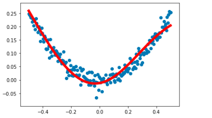
#画图
plt.figure()
plt.scatter(x_data,y_data)
plt.plot(x_data,prediction_value,'r-',lw=5)#线宽为5
plt.show()