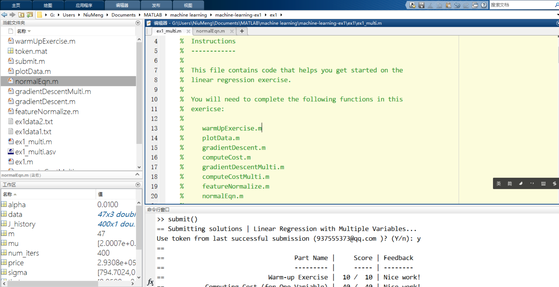
coursera 机器学习 linear regression 线性回归的小项目
Matlab 环境:
1. 一元线性回归
ex1.m
%% Machine Learning Online Class - Exercise 1: Linear Regression
% Instructions
% ------------
%
% This file contains code that helps you get started on the
% linear exercise. You will need to complete the following functions
% in this exericse:
%
% warmUpExercise.m
% plotData.m 绘制房屋面积和房屋价格的点状图
% gradientDescent.m 梯度下降法求theta
% computeCost.m 计算损失函数
% gradientDescentMulti.m
% computeCostMulti.m
% featureNormalize.m 特征缩放
% normalEqn.m 正规方程法求theta
%
% For this exercise, you will not need to change any code in this file,
% or any other files other than those mentioned above.
%
% x refers to the population size in 10,000s
% y refers to the profit in $10,000s
%
%% Initialization
clear ; close all; clc
%% ==================== Part 1: Basic Function ====================
% Complete warmUpExercise.m
fprintf('Running warmUpExercise ... \n');
fprintf('5x5 Identity Matrix: \n');
warmUpExercise()
fprintf('Program paused. Press enter to continue.\n');
pause;
%% ======================= Part 2: Plotting =======================
fprintf('Plotting Data ...\n')
data = load('ex1data1.txt');
X = data(:, 1); y = data(:, 2);
m = length(y); % number of training examples
% Plot Data
% Note: You have to complete the code in plotData.m
plotData(X, y);
fprintf('Program paused. Press enter to continue.\n');
pause;
%% =================== Part 3: Cost and Gradient descent ===================
X = [ones(m, 1), data(:,1)]; % Add a column of ones to x
theta = zeros(2, 1); % initialize fitting parameters
% Some gradient descent settings
iterations = 1500;
alpha = 0.01;
fprintf('\nTesting the cost function ...\n')
% compute and display initial cost
J = computeCost(X, y, theta);
fprintf('With theta = [0 ; 0]\nCost computed = %f\n', J);
fprintf('Expected cost value (approx) 32.07\n');
% further testing of the cost function
J = computeCost(X, y, [-1 ; 2]);
fprintf('\nWith theta = [-1 ; 2]\nCost computed = %f\n', J);
fprintf('Expected cost value (approx) 54.24\n');
fprintf('Program paused. Press enter to continue.\n');
pause;
fprintf('\nRunning Gradient Descent ...\n')
% run gradient descent
theta = gradientDescent(X, y, theta, alpha, iterations);
% print theta to screen
fprintf('Theta found by gradient descent:\n');
fprintf('%f\n', theta);
fprintf('Expected theta values (approx)\n');
fprintf(' -3.6303\n 1.1664\n\n');
% Plot the linear fit
hold on; % keep previous plot visible
plot(X(:,2), X*theta, '-')
legend('Training data', 'Linear regression')
hold off % don't overlay any more plots on this figure
% Predict values for population sizes of 35,000 and 70,000
predict1 = [1, 3.5] *theta;
fprintf('For population = 35,000, we predict a profit of %f\n',...
predict1*10000);
predict2 = [1, 7] * theta;
fprintf('For population = 70,000, we predict a profit of %f\n',...
predict2*10000);
fprintf('Program paused. Press enter to continue.\n');
pause;
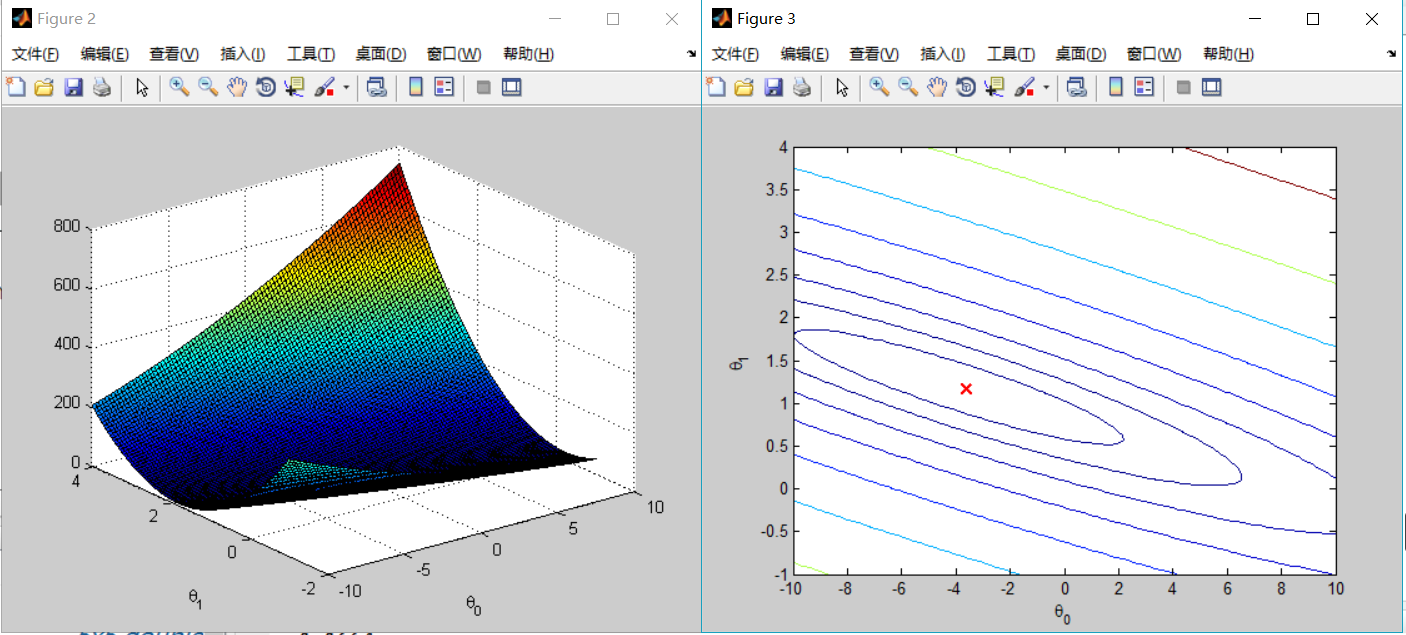
%% ============= Part 4: Visualizing J(theta_0, theta_1) =============
fprintf('Visualizing J(theta_0, theta_1) ...\n')
% Grid over which we will calculate J
theta0_vals = linspace(-10, 10, 100);
theta1_vals = linspace(-1, 4, 100);
% initialize J_vals to a matrix of 0's
J_vals = zeros(length(theta0_vals), length(theta1_vals));
% Fill out J_vals
for i = 1:length(theta0_vals)
for j = 1:length(theta1_vals)
t = [theta0_vals(i); theta1_vals(j)];
J_vals(i,j) = computeCost(X, y, t);
end
end
% Because of the way meshgrids work in the surf command, we need to
% transpose J_vals before calling surf, or else the axes will be flipped
J_vals = J_vals';
% Surface plot
figure;
surf(theta0_vals, theta1_vals, J_vals)
xlabel('\theta_0'); ylabel('\theta_1');
% Contour plot
figure;
% Plot J_vals as 15 contours spaced logarithmically between 0.01 and 100
contour(theta0_vals, theta1_vals, J_vals, logspace(-2, 3, 20))
xlabel('\theta_0'); ylabel('\theta_1');
hold on;
plot(theta(1), theta(2), 'rx', 'MarkerSize', 10, 'LineWidth', 2);

computeCost.m
function J = computeCost(X, y, theta)
%COMPUTECOST Compute cost for linear regression
%   J = COMPUTECOST(X, y, theta) computes the cost of using theta as the
%   parameter for linear regression to fit the data points in X and y

% Initialize some useful values
m = length(y); % number of training examples

% You need to return the following variables correctly
J = 0;

% ====================== YOUR CODE HERE ======================
% Instructions: Compute the cost of a particular choice of theta
%               You should set J to the cost.

h = X * theta ; % cal the hypothesis
J = 1/(2*m) * sum((h-y) .^ 2 ) ;


% =========================================================================

end

gradientDescent.m
function [theta, J_history] = gradientDescent(X, y, theta, alpha, num_iters)
%GRADIENTDESCENT Performs gradient descent to learn theta
%   theta = GRADIENTDESCENT(X, y, theta, alpha, num_iters) updates theta by
%   taking num_iters gradient steps with learning rate alpha

% Initialize some useful values
m = length(y); % number of training examples
J_history = zeros(num_iters, 1);

for iter = 1:num_iters

    % ====================== YOUR CODE HERE ======================
    % Instructions: Perform a single gradient step on the parameter vector
    %               theta.
    %
    % Hint: While debugging, it can be useful to print out the values
    %       of the cost function (computeCost) and gradient here.
    %
h = X * theta ;
h_minus  = h - y;
h_sum = ( h_minus' * X )';
theta = theta - alpha * h_sum ./ m;

    % ============================================================

    % Save the cost J in every iteration
    J_history(iter) = computeCost(X, y, theta);

end

end
多元线性回归
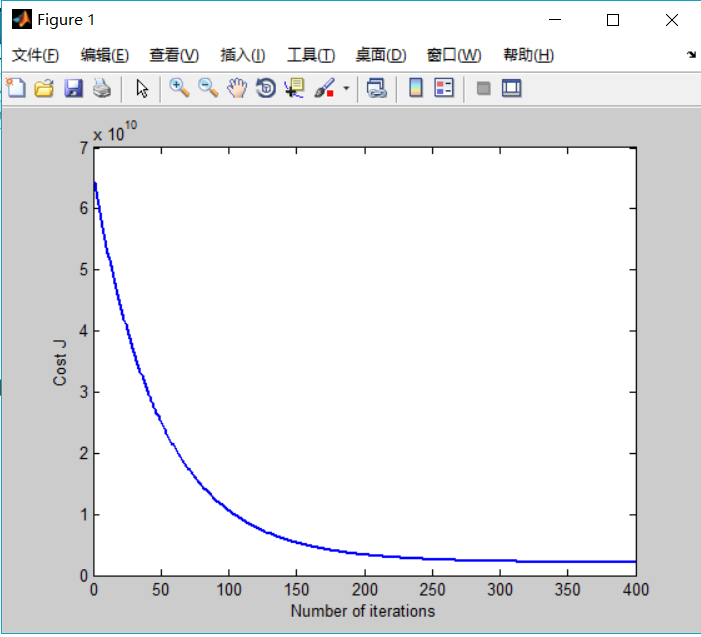
ex1_multi.m
  1 %% Machine Learning Online Class
  2 %  Exercise 1: Linear regression with multiple variables
  3 %
  4 %  Instructions
  5 %  ------------
  6 %
  7 %  This file contains code that helps you get started on the
  8 %  linear regression exercise.
  9 %
 10 %  You will need to complete the following functions in this
 11 %  exericse:
 12 %
 13 %     warmUpExercise.m
 14 %     plotData.m
 15 %     gradientDescent.m
 16 %     computeCost.m
 17 %     gradientDescentMulti.m
 18 %     computeCostMulti.m
 19 %     featureNormalize.m
 20 %     normalEqn.m
 21 %
 22 %  For this part of the exercise, you will need to change some
 23 %  parts of the code below for various experiments (e.g., changing
 24 %  learning rates).
 25 %
 26
 27 %% Initialization
 28
 29 %% ================ Part 1: Feature Normalization ================
 30
 31 %% Clear and Close Figures
 32 clear ; close all; clc
 33
 34 fprintf('Loading data ...\n');
 35
 36 %% Load Data
 37 data = load('ex1data2.txt');
 38 X = data(:, 1:2);
 39 y = data(:, 3);
 40 m = length(y);
 41
 42 % Print out some data points
 43 fprintf('First 10 examples from the dataset: \n');
 44 fprintf(' x = [%.0f %.0f], y = %.0f \n', [X(1:10,:) y(1:10,:)]');
 45
 46 fprintf('Program paused. Press enter to continue.\n');
 47 pause;
 48
 49 % Scale features and set them to zero mean
 50 fprintf('Normalizing Features ...\n');
 51
 52 [X mu sigma] = featureNormalize(X);
 53
 54 % Add intercept term to X
 55 X = [ones(m, 1) X];
 56
 57
 58 %% ================ Part 2: Gradient Descent ================
 59
 60 % ====================== YOUR CODE HERE ======================
 61 % Instructions: We have provided you with the following starter
 62 %               code that runs gradient descent with a particular
 63 %               learning rate (alpha).
 64 %
 65 %               Your task is to first make sure that your functions -
 66 %               computeCost and gradientDescent already work with
 67 %               this starter code and support multiple variables.
 68 %
 69 %               After that, try running gradient descent with
 70 %               different values of alpha and see which one gives
 71 %               you the best result.
 72 %
 73 %               Finally, you should complete the code at the end
 74 %               to predict the price of a 1650 sq-ft, 3 br house.
 75 %
 76 % Hint: By using the 'hold on' command, you can plot multiple
 77 %       graphs on the same figure.
 78 %
 79 % Hint: At prediction, make sure you do the same feature normalization.
 80 %
 81
 82 fprintf('Running gradient descent ...\n');
 83
 84 % Choose some alpha value
 85 alpha = 0.01;
 86 num_iters = 400;
 87
 88 % Init Theta and Run Gradient Descent
 89 theta = zeros(3, 1);
 90 [theta, J_history] = gradientDescentMulti(X, y, theta, alpha, num_iters);
 91
 92 % Plot the convergence graph
 93 figure;
 94 plot(1:numel(J_history), J_history, '-b', 'LineWidth', 2);
 95 xlabel('Number of iterations');
 96 ylabel('Cost J');
 97
 98 % Display gradient descent's result
 99 fprintf('Theta computed from gradient descent: \n');
100 fprintf(' %f \n', theta);
101 fprintf('\n');
102
103 % Estimate the price of a 1650 sq-ft, 3 br house
104 % ====================== YOUR CODE HERE ======================
105 % Recall that the first column of X is all-ones. Thus, it does
106 % not need to be normalized.
107 price = 0; % You should change this
108 X_1 = [1 1650 3] ;
109 price  = X_1 * theta ;
110 % ============================================================
111
112 fprintf(['Predicted price of a 1650 sq-ft, 3 br house ' ...
113          '(using gradient descent):\n $%f\n'], price);
114
115 fprintf('Program paused. Press enter to continue.\n');
116 pause;
117
118 %% ================ Part 3: Normal Equations ================
119
120 fprintf('Solving with normal equations...\n');
121
122 % ====================== YOUR CODE HERE ======================
123 % Instructions: The following code computes the closed form
124 %               solution for linear regression using the normal
125 %               equations. You should complete the code in
126 %               normalEqn.m
127 %
128 %               After doing so, you should complete this code
129 %               to predict the price of a 1650 sq-ft, 3 br house.
130 %
131
132 %% Load Data
133 data = csvread('ex1data2.txt');
134 X = data(:, 1:2);
135 y = data(:, 3);
136 m = length(y);
137
138 % Add intercept term to X
139 X = [ones(m, 1) X];
140
141 % Calculate the parameters from the normal equation
142 theta = normalEqn(X, y);
143
144 % Display normal equation's result
145 fprintf('Theta computed from the normal equations: \n');
146 fprintf(' %f \n', theta);
147 fprintf('\n');
148
149
150 % Estimate the price of a 1650 sq-ft, 3 br house
151 % ====================== YOUR CODE HERE ======================
152 price = 0; % You should change this
153 X_2 = [ 1 1650 3] ;
154 price  = X_2 * theta ;
155 % ============================================================
156
157 fprintf(['Predicted price of a 1650 sq-ft, 3 br house ' ...
158          '(using normal equations):\n $%f\n'], price);
特征缩放
 1 function [X_norm, mu, sigma] = featureNormalize(X)
 2 %FEATURENORMALIZE Normalizes the features in X
 3 %   FEATURENORMALIZE(X) returns a normalized version of X where
 4 %   the mean value of each feature is 0 and the standard deviation
 5 %   is 1. This is often a good preprocessing step to do when
 6 %   working with learning algorithms.
 7
 8 % You need to set these values correctly
 9 X_norm = X;
10 mu = zeros(1, size(X, 2));
11 sigma = zeros(1, size(X, 2));
12
13 % ====================== YOUR CODE HERE ======================
14 % Instructions: First, for each feature dimension, compute the mean
15 %               of the feature and subtract it from the dataset,
16 %               storing the mean value in mu. Next, compute the
17 %               standard deviation of each feature and divide
18 %               each feature by it's standard deviation, storing
19 %               the standard deviation in sigma.
20 %
21 %               Note that X is a matrix where each column is a
22 %               feature and each row is an example. You need
23 %               to perform the normalization separately for
24 %               each feature.
25 %
26 % Hint: You might find the 'mean' and 'std' functions useful.
27 %
28 mu = mean(X); % 1 * ( n + 1 )
29 sigma = std(X);
30 for i = 1 : size(X,1)
31     X_norm(i,:) = ( X_norm(i,:) - mu ) ./ sigma ; % 对每个行向量做减法
32 end
33 %  X_norm(1:10,:)
34
35 % ============================================================
36
37 end
computeCostMulti and gradientDescent是没有变的。
正规方程法
 1 function [theta] = normalEqn(X, y)
 2 %NORMALEQN Computes the closed-form solution to linear regression
 3 %   NORMALEQN(X,y) computes the closed-form solution to linear
 4 %   regression using the normal equations.
 5
 6 theta = zeros(size(X, 2), 1);
 7
 8 % ====================== YOUR CODE HERE ======================
 9 % Instructions: Complete the code to compute the closed form solution
10 %               to linear regression and put the result in theta.
11 %
12
13 % ---------------------- Sample Solution ----------------------
14
15 theta = pinv(X'*X)*X'*y;
16
17
18 % -------------------------------------------------------------
19
20
21 % ============================================================
22
23 end

源码:
https://github.com/twomeng/linear-regression-

 浙公网安备 33010602011771号