


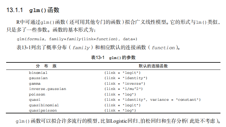

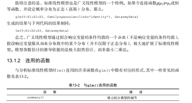


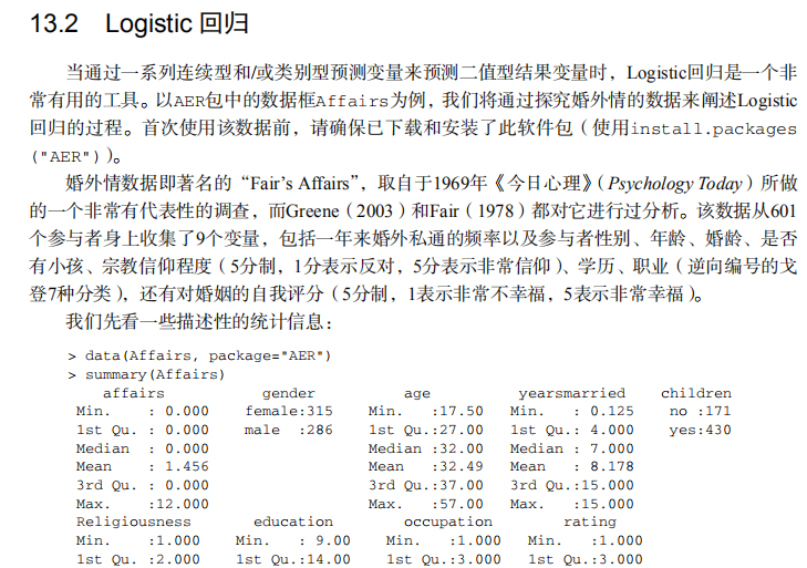
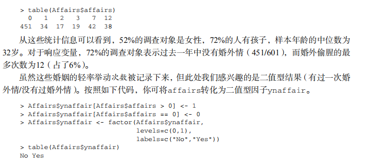
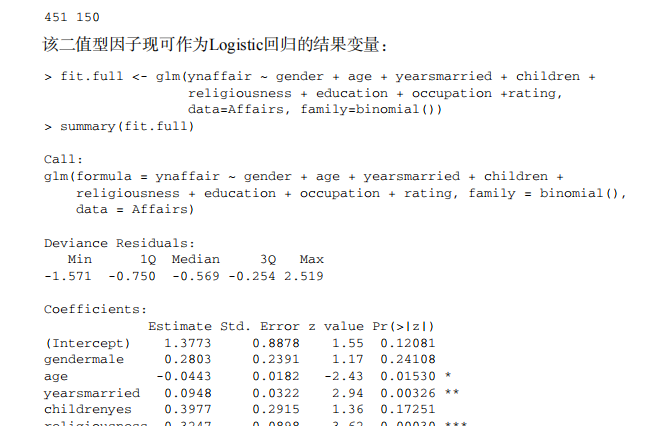


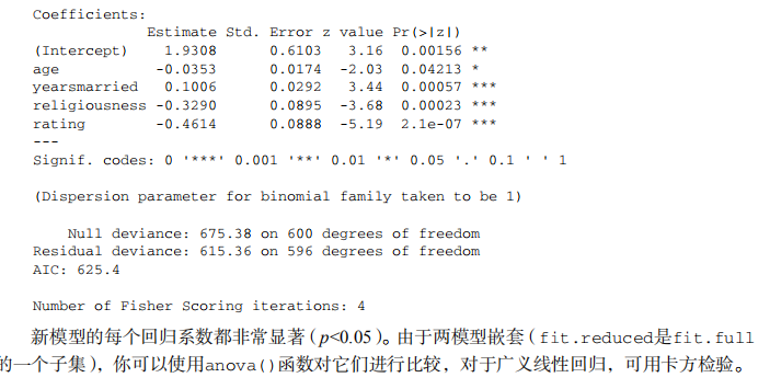
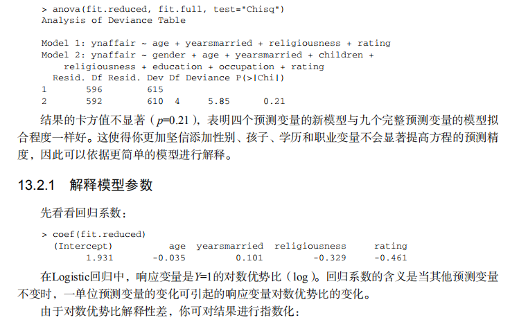


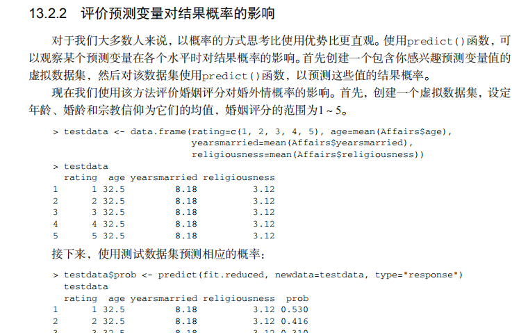

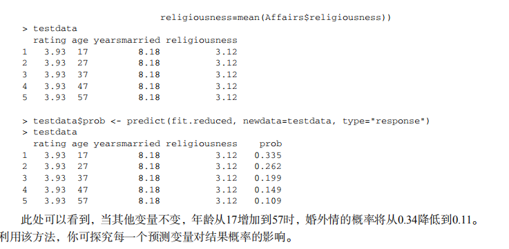
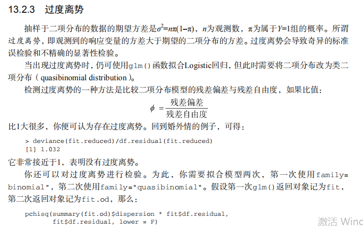

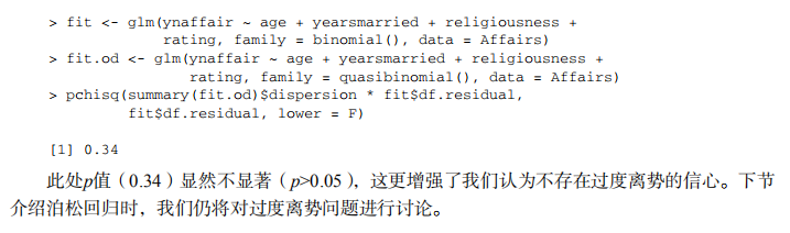
#----------------------------------------------#
# R in Action (2nd ed): Chapter 13             #
# Generalized linear models                    #
# requires packages AER, robust, gcc           #
# install.packages(c("AER", "robust", "gcc"))  #
#----------------------------------------------#


## Logistic Regression

# get summary statistics
data(Affairs, package="AER")
summary(Affairs)
table(Affairs$affairs)

# create binary outcome variable
Affairs$ynaffair[Affairs$affairs > 0] <- 1
Affairs$ynaffair[Affairs$affairs == 0] <- 0
Affairs$ynaffair <- factor(Affairs$ynaffair,
                           levels=c(0,1),
                           labels=c("No","Yes"))
table(Affairs$ynaffair)

# fit full model
fit.full <- glm(ynaffair ~ gender + age + yearsmarried + children +
                  religiousness + education + occupation +rating,
                data=Affairs,family=binomial())
summary(fit.full)

# fit reduced model
fit.reduced <- glm(ynaffair ~ age + yearsmarried + religiousness +
                     rating, data=Affairs, family=binomial())
summary(fit.reduced)

# compare models
anova(fit.reduced, fit.full, test="Chisq")

# interpret coefficients
coef(fit.reduced)
exp(coef(fit.reduced))

# calculate probability of extramariatal affair by marital ratings
testdata <- data.frame(rating = c(1, 2, 3, 4, 5),
                       age = mean(Affairs$age),
                       yearsmarried = mean(Affairs$yearsmarried),
                       religiousness = mean(Affairs$religiousness))
testdata$prob <- predict(fit.reduced, newdata=testdata, type="response")
testdata

# calculate probabilites of extramariatal affair by age
testdata <- data.frame(rating = mean(Affairs$rating),
                       age = seq(17, 57, 10),
                       yearsmarried = mean(Affairs$yearsmarried),
                       religiousness = mean(Affairs$religiousness))
testdata$prob <- predict(fit.reduced, newdata=testdata, type="response")
testdata

# evaluate overdispersion
fit <- glm(ynaffair ~ age + yearsmarried + religiousness +
             rating, family = binomial(), data = Affairs)
fit.od <- glm(ynaffair ~ age + yearsmarried + religiousness +
                rating, family = quasibinomial(), data = Affairs)
pchisq(summary(fit.od)$dispersion * fit$df.residual,
       fit$df.residual, lower = F)


## Poisson Regression

# look at dataset
data(breslow.dat, package="robust")
names(breslow.dat)
summary(breslow.dat[c(6, 7, 8, 10)])

# plot distribution of post-treatment seizure counts
opar <- par(no.readonly=TRUE)
par(mfrow=c(1, 2))
attach(breslow.dat)
hist(sumY, breaks=20, xlab="Seizure Count",
     main="Distribution of Seizures")
boxplot(sumY ~ Trt, xlab="Treatment", main="Group Comparisons")
par(opar)

# fit regression
fit <- glm(sumY ~ Base + Age + Trt, data=breslow.dat, family=poisson())
summary(fit)

# interpret model parameters
coef(fit)
exp(coef(fit))

# evaluate overdispersion
deviance(fit)/df.residual(fit)
library(qcc)
qcc.overdispersion.test(breslow.dat$sumY, type="poisson")

# fit model with quasipoisson
fit.od <- glm(sumY ~ Base + Age + Trt, data=breslow.dat,
              family=quasipoisson())
summary(fit.od)
