『笔记』LSS

『笔记』LSS

1 Introduction

Computer vision algorithms generally take as input an image and output either a prediction that is coordinate-frame agnostic. This paradigm does not match the setting for perception in self-driving out- of-the-box. In self-driving, multiple sensors are given as input, each with a dif- ferent coordinate frame, and perception models are ultimately tasked with producing predictions in a new coordinate frame – the frame of the ego car

We propose a model named “Lift-Splat” that preserves the 3 symmetries (pixel-transition equivariance, camera-permutation invariance, ego-frame isometry equivariance) identified above by design while also being end-to-end differentiable.

3 Method

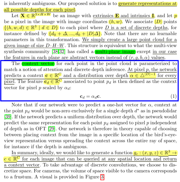
Formally, we are given n images \(\{X_k \in \mathbb{R}^{3×H×W}\}_n\) each with an extrinsic matrix \(E_k \in \mathbb{R}^{3×4}\) and an intrinsic matrix \(I_k \in \mathbb{R}^{3×3}\), and we seek to find a rasterized representation of the scene in the BEV coordinate frame \(y ∈ \mathbb{R}^{C×X×Y}\) . The extrinsic and intrinsic matrices together define the mapping from reference coordinates \((x, y, z)\) to local pixel coordinates \((h, w, d)\) for each of the n cameras.

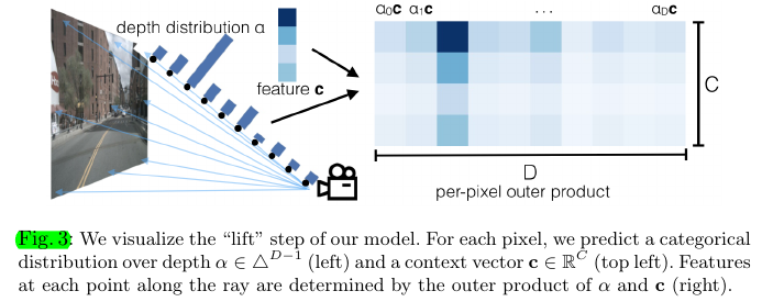
3.1 Lift: Latent Depth Distribution

The purpose of this stage is to “lift” each image from a local 2-dimensional coordinate system to a 3-dimensional frame

3.2 Splat: Pillar Pooling

We follow the pointpillars [18] architecture to convert the large point cloud output by the “lift” step. We assign every point to its nearest pillar and perform sum pooling to create a \(C × H × W\) tensor

Just as OFT [29] uses integral images to speed up their pooling step, we apply an analagous technique to speed up sum pooling. Efficiency is crucial for training our model given the size of the point clouds generated. Instead of padding each pillar then performing sum pooling, we avoid padding by using packing and leveraging a "cumsum trick" for sum pooling. This operation has an analytic gradient that can be calculated efficiently to speed up autograd as explained in subsection 4.2.

3.3 Shoot: Motion Planning

[skip]

4 Implementation

4.1 Architecture Details

[...]

There are several hyper-parameters that determine the “resolution” of our model. First, the size of the input images \(H × W\). In all experiments below, we resize and crop input images to size 128 × 352 and adjust extrinsics and intrinsics accordingly. Another important hyperparameter is the size and resolution of the bev grid \(X × Y\). In our experiments, we set bins in both \(x\) and \(y\) from -50 meters to 50 meters with cells of size 0.5 meters × 0.5 meters. The resultant grid is therefore 200×200. Finally, there’s the choice of \(D\) that determines the resolution of depth predicted by the network. We restrict \(D\) between 4.0 meters and 45.0 meters spaced by 1.0 meters.

4.2 Frustum Pooling Cumulative Sum Trick

Training efficiency is critical for learning from data from an entire sensor rig. We choose sum pooling across pillars in Section 3 as opposed to max pooling because our “cumulative sum” trick saves us from excessive memory usage due to padding.

The "cumulative sum trick" is the observation that sum pooling can be performed by sorting all points according to bin id, performing a cumulative sum over all features, then subtracting the cumulative sum values at the boundaries of the bin sections. Instead of relying on autograd to backprop through all three steps, the analytic gradient for the module as a whole can be derived, speeding up training by 2x.

We call the layer "Frustum Pooling" because it handles converting the frustums produced by n images into a fixed dimensional \(C × H × W\) tensor independent of the number of cameras \(n\).