『笔记』快速recap CS4240主要知识

『笔记』快速recap CS4240主要知识

1.1 Logistics & 1.2 Feedforward

Deep feed forward networks: approximate some function f*

Training a network: 1. present a training sample, 2. compare the results, 3. update the weights.

Minimize some criterion. Reduce loss: moving in the opposite sign (gradient descent, GD). View those params as the decision variable of the cost function. Gradient: a vector of all partial derivatives

SGD: an approximation of the gradient from a small number of samples

Activation function: add non-linearity. ReLU

2.1 MLrefresh & 2.2 Backprop

Maximum likelihood estimation

We would like to have some principles from which we can derive specific functions that are good estimators for different models => most common: max likelihood

A set of examples \(\mathbb{X}=\{x^{(1)}, ..., x^{(m)}\}\) drawn independently from the true but unknown distribution \(p_{\text{data}}(x)\). \(p_\text{model}(x;\theta)\) is a parametric family of probability distributions that maps any \(x\) to a real number estimating the true probability \(p_{\text{data}}(x)\)

\[\theta_{ML} = \underset{\theta}{\text{argmax}} \space p_{\text{model}}(\mathbb{X};\theta) = \underset{\theta}{\text{argmax}} \prod_{i=1}^m p_{\text{model}}(x^{(i)};\theta) \]

\[\overset{1}{\rightarrow} \underset{\theta}{\text{argmax}} \sum_{i=1}^m \log p_{\text{model}}(x^{(i)};\theta) \overset{2}{\rightarrow} \underset{\theta}{\text{argmax}} \space \mathbb{E}_{x\sim\hat{p}_{\text{data}}} \log p_{\text{model}}(x;\theta) \]

1. Accumulate mutiplication is inconvenient because unstable close to 0 numerically, so use log to convert it to be summation.
2. Argmax does not change if rescale, we divide by \(m\) to obtan a version expressed as an expectation with respect to the empirical distribution \(\hat{p}_{\text{data}}\)

在我们参数化的\(p_{\text{model}}\)中，从真实的\(p_{\text{data}}\)下sample出来的样本们有了最大的概率，因为大概率的样本更容易被真实的\(p_{\text{data}}\)采样出来，这样就让我们的\(p_{\text{model}}\)逼近了\(p_{\text{data}}\). 所以，minimize dissimilarity between \(p_{\text{model}}\) and \(p_{\text{data}}\)

于是另一个角度：measure the dissimilarity by KL divergence

\[D(p_{\text{data}} || p_{\text{model}}) = \sum_{i=1}^m \hat{p}_{\text{data}}(x^{(i)}) \log(\frac{\hat{p}_{\text{data}}(x^{(i)})}{p_{\text{model}}(x^{(i)})}) = \sum_{i=1}^m \hat{p}_{\text{data}}(x^{(i)}) (\log{\hat{p}_{\text{data}}(x^{(i)})} - \log {p_{\text{model}}(x^{(i)})}) \]

\[\rightarrow \mathbb{E}_{x\sim\hat{p}_{\text{data}}} (\log{\hat{p}_{\text{data}}(x)} - \log {p_{\text{model}}(x)}) \rightarrow \mathbb{E}_{x\sim\hat{p}_{\text{data}}} -\log {p_{\text{model}}(x)} \]

所以minimize KL divergence得到的式子和maximize likelihood是一个意思

Cross-entrophy

Cross-entrophy: a generic term.

Any loss consisting of a negative log-likelihood is a cross-entrophy between the empirical probability distribution defined by the training set (label) and the probability distribution defined by the model (prediction)

核心组成即negative log-likelihood，核心思路即想要用有CE组成的这个loss function来让我们的模型预测概率分布迫近与所能拿到的训练集的概率分布。这几个概念等价的：maximize maximum likelihood, minimize KL divergence, minimize negative log-likelihood, minimize cross-entrophy

Conditional log-likelihood and output units

Output units determine the form of the cross-entrophy function

The maximum likelihood can be readily generalized to estimate a conditional probability \(p(\mathbb{Y}|\mathbb{X};\theta)\) to predict \(y\) given \(x\):

\[\theta_{ML} = \underset{\theta}{\text{argmax}} \space p_{\text{model}}(\mathbb{Y}|\mathbb{X};\theta) = \underset{\theta}{\text{argmax}} \sum_{i=1}^m \log p_{\text{model}}(y^{(i)} | x^{(i)};\theta) \]

Binary/multi classification

Binary classification / logistic regression (binary label, sigmoid, binary CE)
Multi-class classification (one-hot encoding, softmax, CE)

	Label distribution	Activation	Loss function
BC/LR	Bernoulli distribution: \(t\in\{0,1\}\)	Sigmoid: \(y=\sigma(z)=\frac{1}{1+e^{-z}}\)	Binary CE: \(\mathcal{L}(y,t)=-t\log y-(1-t)\log (1-y)\)
MC	One-hot encoding: \(t=(0, ...,0, 1, 0, ..., 0)\)	Softmax: \(y_k=\frac{e^{z_k}}{\sum_{k^\prime}e^{z_{k^\prime}}}\)	Multi-class CE: \(\mathcal{L}(y,t)=-\sum_{k=1}^K t_k \log y_k =-t^T\log y\)

• Activation的作用：为了归一化在[0,1]内，毕竟要作为CE的用法是probability
• 相比MSE，CE能够penalize really wrong predictions CE产生的效果（回忆Binary CE那个对称的双曲线）

另外，Softmax函数和Sigmoid函数的区别与联系

Backward pass: Back-propagation

Backpropagation is a clever application of the chain rule of calculus updating the weights.

Q: How does “1-d” example plot change to a multi-layer network?
A: One coordinate for each weight/bias

Chain rule to compute derivatives

Leibniz notation: \(\frac{dz}{dx}=\frac{dz}{dy}\frac{dy}{dx}\). "How much does the output change if the input slightly changes"

“Bar notation”: for computed values: \(\overline{y}=\frac{d\mathcal{L}}{dy}\)，即最终的loss对该值的偏导

Computational graph: topological ordering

拓扑排序（Topological ordering）: linear ordering of vertices, so for every directed edge \(uv\), vertex \(u\) comes before \(v\) in the ordering. 在我们的情况下，vertex (node): variable, scalar, vector, matrix, tensor, etc. edge (operation): a single function

Backward pass:

\[\overline{n}_N=1 \]

\[\overline{n}_i = \sum _{n_j \in \text{children}(n_i)}\overline{n}_j \frac{\partial n_j}{\partial n_i} \quad \text{for} \space i=N-1, ..., 1 \]

所以，如上所示可以总结为每一次的计算的目标就是对该过程（边）的input（结点）求bar notation，方式是1. aggregates the error signal from all its children 2. 基于每个child \(n_j\)的已经传过来的计算好的它的bar notation，根据当前\(i\)与这个\(j\)所连的这条具体的边，在其上叠加本步过程边的偏导\(\frac{\partial n_j}{\partial n_i}\)

3.1 CNN part 1 & 3.2 CNN part 2

Convolution: moving neighborhood average generalized to a kernel

A bit of image processing: how to get rid of noisy pixels? moving neighborhood average

Design a color coding: flower & Waldo example. So kernel weights are feature detectors, so learning weights = learning features, and so, ConvNets learns the feature representation

Convolutional network

Different kernels/filters act as different kind of feature extractors (所以设置这么多有用，可以拥有不同的pattern)

Spatial pooling: 1. summarizes the outcomes over a region 2. after downsampling we can see larger features 3. reducing memory. We do not need to store all backprop information.

Padding: avoid losing boundary, prevent shrinking

Convolutional versus feed forward

Convolution operation could be written as a matrix multiplication using Toeplitz matrix, which is 1. sparse (many zeros) 2. local (non-zero values occur next to each other) 3. sharing params (same values repeat). So CNN is by-design a limited parameter version of feed forward. Why use it? curse of dimensionality

Convolution's equivariance

Equivariance: \(f(g(x))=g(f(x))\). Conv then translating = translating then conv. So for CNN the object locations does not matter

Pooling's invariance

Invariance: \(f(g(x))=f(x)\). So for pooling, feature presence more important than feature location

Receptive field

How much does the shaded neuron “see” the image?

Convolution increases RF linearly, pooling multiplicatively

Exercise: compute the number of parameters.
Exercise: compute the receptive of field.

4 Regularization

Overfitting

Overfitting: the gap between true error (on test set) and apparent error (on training set)

Plots: error vs. training set size (not the same as training process of a neural net!)

• Training set size ++, overfitting --
• model complexity --, overfitting --

Bayes error

Beating overfitting

Data augmentation (more data!)

Regularization: techniques to reduce the test error, possibly at the expense of increased training error

• Feature reduction: a bit out of fashion. Sometime sneakily done in image classification
• Reduce complexity / flexibility of the model

Reduce complexity / flexibility of the model

Generalization bounds: a formula predicting the possible latent upper gap to touch the true error

• Number of layers & absolute value of weights -> larger, the upper bound higher (可能的test error加的越高)

Parameter norm regularization: l1 / l2 norm; not only move on the negative direction on the loss curve, also on the weights

Early stopping: useful when network is correctly initialized

Weight space

(Noise robustness: noise added to inputs/weights/outputs)

Parameter sharing / tying

Dropout: each training loop, randomly select a fraction of the nodes, and make them inactive (zero)

• Works for “wide” but not for “deep and slim” networks
• Not suitable for cnn (apply on fc layer)

5 Optimization

Tuning the learning rate

Eclipse: contour plot, altitude map. A dot: a particular parameter set
Too high: never found a good instantiation
Too low: take very long to find a good instantiation
Q: Going backward? A: because we use small batches to approximately represent the gradient over the whole set. And the map here is the actual, true loss map. So sometimes even going backwards. If we use the whole set, the trajectory will strictly follow the map

Reduce LR over time (decay) (learning rate schedule)

Exponentially weighted moving average (EWMA):

EWMA: A memory efficient approach to compute summary statistics online.
For value \(y_t\) at time \(t\), \(\rho \in [0, 1]\), \(S_0=0\)

\[S_t=\rho S_{t-1}+(1-\rho)y_t \]

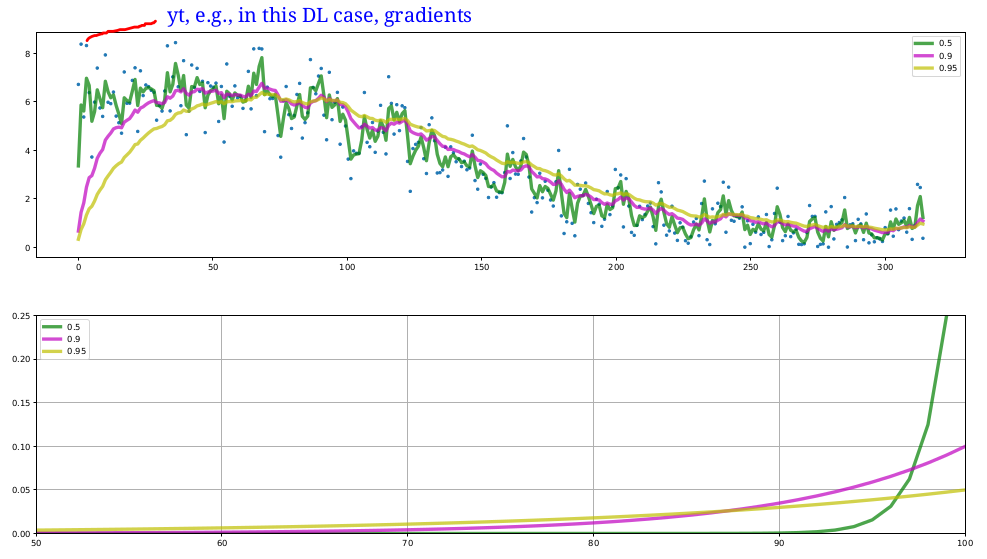
• upper plot: shows the overall process
• bottom plot: shows the contributions composing \(S_{100}\)

在我们的情况下，\(y_t\)就是gradient

Bias correction

Notice the difference at the beginning: the larger \(\rho\) is, the later it "catches up". 对过去的记忆太大，于是在初始值时问题较大，因为从零开始

Bias correction: \(\hat{S_t}=\frac{S_t}{1-\rho ^t}\)

When \(t\) is large, \(1-\rho t=1\), so \(\hat{S_t}=S_t\), bias correction influence gradually decreases

SGD with Momentum, RMSProp and Adam

Hey man, I'm in the deep learning course, I want to learn about those algorithms!

SGD with Momentum

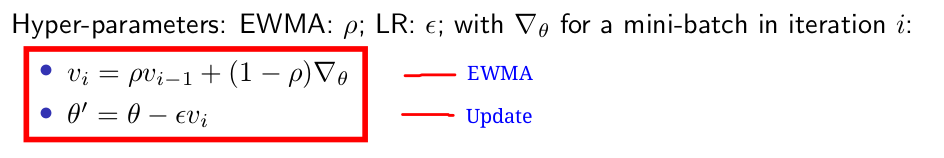
Often implemented without bias correction, default setting \(\rho=0.9\)

SGD with RMSProp

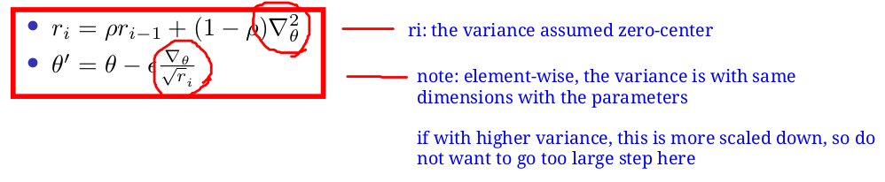
To prevent dividing by 0, add a small \(\delta=10^{-6}\) to denominator: \(r_i=\delta+r_i\)
Often implemented without bias correction, default setting \(\rho=0.9\)

SGD with Adam

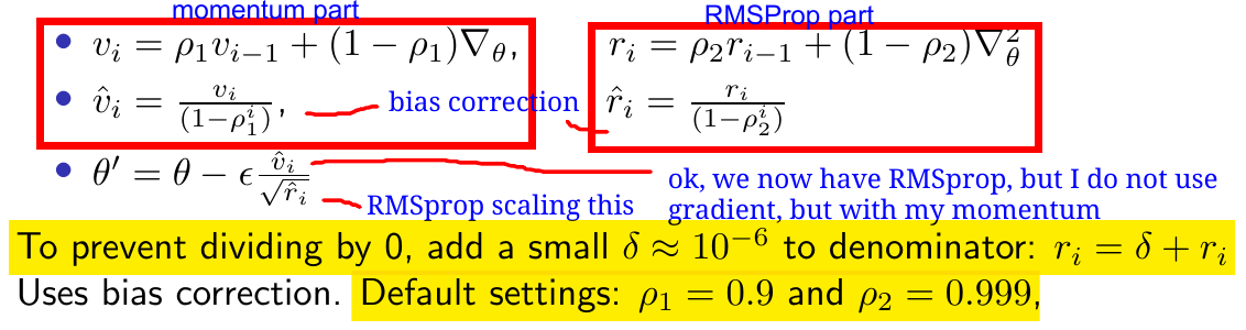
“Average” and “variance”:
- SGD with Momentum: smooths the average of noisy gradients by EWMA (就是EWMA的思想和作用)
- SGD with RMSprop: smooths the zero-centered variance (在大variance的维度上就会驱使走小一点)
- Adam: momentum + rmsprop + bias correction

Effect of feature normalization on optimization

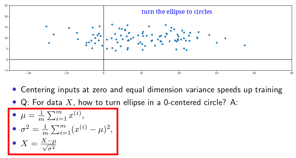
centering inputs at zero and equal dimension variance speeds up training

Batch norm: normalizing learned features

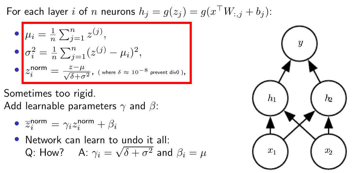
At test time: use the weighted average for \(\mu, \sigma^2\) to compute and \(\gamma,\beta\) to compute batch-normed sample. i.e., maintain a EMWA over batches when we are training

https://myrtle.ai/how-to-train-your-resnet-7-batch-norm/
The good

• it stabilises optimisation allowing much higher learning rates and faster training
• it injects noise (through the batch statistics) improving generalisation
• it reduces sensitivity to weight initialisation
• it interacts with weight decay to control the learning rate dynamics

The bad

• t’s slow (although node fusion can help)
• it’s different at training and test time and therefore fragile
• it’s ineffective for small batches and various layer types
• it has multiple interacting effects which are hard to separate.

6 Recurrent neural networks (RNNs)

7 Self-attention

关于transformer的内容自己在另外两个post里已经专心总结了，在这里这一章就保持简短总结

Previously RNN uses a recurrent way to get some relationships between words (pass the info through), e.g., students, …, were. Now if we want parallel training, how we can do? A: Link each word to each other word

Learning how to re-weight with all other words. A sequence-to-sequence operation. How to determine how much a word A can re-weight a word B? A: some similarity (e.g., dot product \(\textbf{x}_i^T\textbf{x}_j\))

Self-attention

Each vector \(x_i\) is used in three roles: queries, keys, values. Query: for its own weights, compared to others. Key: for other vectors weights. Values: as a part of the weighted sum for the output
\(W_q\) and \(W_k\) added in the dot-product (similarity). \(W_v\) added in the summing

Mutil-head attention: represent multiple relations a word can have

Narrow & wide

Position embedding

Q: If I change the word order, do I get different results?
A: No, dot-product and sum is permutation invariant

Position embedding & position encoding

8 Unsupervised

...