『笔记』二维目标检测的部分基础笔记

『笔记』二维目标检测部分基础笔记

Useful links

• CS4245 Lecture 5 notes
• CS4245 seminar paper Mask R-CNN notes
• YOLO-从零开始入门目标检测
• 一文读懂Faster RCNN
• 捋一捋pytorch官方FasterRCNN代码
• 令人拍案称奇的Mask RCNN
• mAP (mean Average Precision) for Object Detection
• 目标检测里的多尺度技术
• 如何评价旷视开源的YOLOX，效果超过YOLOv5?
• 一位算法工程师从30+场秋招面试中总结出的目标检测算法面经（含答案）
• 目标检测回归损失函数——IOU、GIOU、DIOU、CIOU、EIOU

Basics

Basic approach: sliding window + binary classifier

Slide window over locations + sizes, following by a binary classifier to judge car or not

Classification+Localization: How should we arrange the labels?

• y1 = [P_c, x, y, w, h, C_1, C_2, C_3] = [1, x, y, w, h, C_1, C_2, C_3]
• y2 = [P_c, x, y, w, h, C_1, C_2, C_3] = [0, x, y, w, h, C_1, C_2, C_3]
• P_c = 0, then the rest fields are not needed because there is no object
• Note:
  • P_c: Is there an object in the patch / window (is there or not)
  • x, y, w, h: bounding box
  • C_1, C_2, C_3: confidence scores of the corresponding classes

NMS (and IoU):

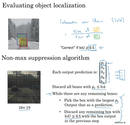
Likely the model is able to find multiple bounding boxes for the same object. Non-max suppression helps avoid repeated detection of the same instance. 个人理解NMS步骤：

• (Suppose only one class is considered) After we get a set of matched bounding boxes for the same object category: Sort all the bounding boxes by confidence score.
  • Discard boxes with low confidence scores. Then
  • Repeat the following: greedily select the one with the highest score and discard the remaining boxes with high IoU (i.e. > 0.5) with the selected one. Do this process until there is no remaining bounding box.
• If multi-classes, do the process class-wise (for each class, and the confidence score will be P_c * C_i)

def nms(self, dets, scores):
        # 这是一个最基本的基于python语言的nms操作
        # 这一代码来源于Faster RCNN项目
        """"Pure Python NMS baseline."""
        x1 = dets[:, 0]  #xmin
        y1 = dets[:, 1]  #ymin
        x2 = dets[:, 2]  #xmax
        y2 = dets[:, 3]  #ymax

        areas = (x2 - x1) * (y2 - y1)                    # bbox的宽w和高h
        order = scores.argsort()[::-1]                   # 按照降序对bbox的得分进行排序

        keep = []                                        # 用于保存经过筛的最终bbox结果
        while order.size > 0:
            i = order[0]                                 # 得到最高的那个bbox
            keep.append(i)                               
            xx1 = np.maximum(x1[i], x1[order[1:]])
            yy1 = np.maximum(y1[i], y1[order[1:]])
            xx2 = np.minimum(x2[i], x2[order[1:]])
            yy2 = np.minimum(y2[i], y2[order[1:]])

            w = np.maximum(1e-28, xx2 - xx1)
            h = np.maximum(1e-28, yy2 - yy1)
            inter = w * h

            # Cross Area / (bbox + particular area - Cross Area)
            ovr = inter / (areas[i] + areas[order[1:]] - inter)
            #reserve all the boundingbox whose ovr less than thresh
            inds = np.where(ovr <= self.nms_thresh)[0]
            order = order[inds + 1]

        return keep

Hard Negative Mining

• We consider bounding boxes without objects as negative examples. Not all the negative examples are equally hard to be identified. For example, if it holds pure empty background, it is likely an “easy negative”; but if the box contains weird noisy texture or partial object, it could be hard to be recognized and these are “hard negative”
• The hard negative examples are easily mis-classified. We can explicitly find those false positive samples during the training loops and include them in the training data so as to improve the classifier

Backbone, neck and head

• 《目标检测》-第2章-Backbone与Detection head

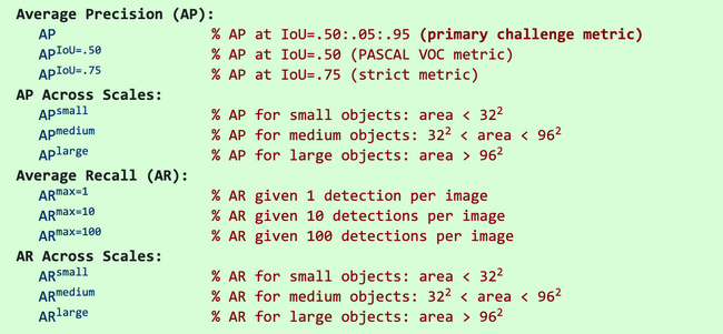
COCO benchmark

Latest research papers tend to give results for the COCO dataset only. In COCO mAP, a 101-point interpolated AP definition is used in the calculation. For COCO, AP is the average over multiple IoU (the minimum IoU to consider a positive match). AP@[.5:.95] corresponds to the average AP for IoU from 0.5 to 0.95 with a step size of 0.05. For the COCO competition, AP is the average over 10 IoU levels on 80 categories (AP@[.50:.05:.95]: start from 0.5 to 0.95 with a step size of 0.05). The following are some other metrics collected for the COCO dataset.

And, this is the AP result for the YOLOv3 detector.

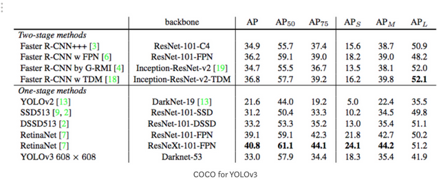
In the figure above, AP@.75 means the AP with IoU=0.75.

mAP (mean average precision) is the average of AP. In some context, we compute the AP for each class and average them. But in some context, they mean the same thing. For example, under the COCO context, there is no difference between AP and mAP. Here is the direct quote from COCO:

AP is averaged over all categories. Traditionally, this is called “mean average precision” (mAP). We make no distinction between AP and mAP (and likewise AR and mAR) and assume the difference is clear from context.

In ImageNet, the AUC method is used. So even all of them follow the same principle in measurement AP, the exact calculation may vary according to the datasets. Fortunately, development kits are available in calculating this metric.