

ChaLearn Gesture Challenge_3:Approximated gradients源码简单分析
前言
上一篇博文ChaLearn Gesture Challenge_2:examples体验 中简单介绍了CGC官网提供的丰富的sample,本节来简单分下其中的一个sample源码,该sample也是examples下的一个,即计算图像的近似梯度图。(其实如果熟悉matlab的朋友应该觉得这个例子很简单,只是本人由于很少使用matlab编写代码,一些基础的东西并没接触过。所以分析这个简单的代码照样可以收获很多matlab基础知识)。
开发环境:matlab2012a
实验基础
首先来看看本例子代码中所需要用到的一些matlab函数和一些基础知识点:
1. evalResponse = input(prompt)
后台上显示prompt的内容,且等待用户键盘输入,输入值保存在evalResponse变量中。
2. .mat文件经过load后,可以在workspace中双击该文件名查看文件中的变量的值,因为.mat里面全部存储的是数据。本程序中的alignment.mat文件中包含了2个变量,分别为alignment_annotation和alignment_labels,两者都是1个1*260的结构。
3. tline = fgetl(fileID)
fileID是通过fopen函数打开文件后得到的一个整型的文件标识。fgetl从这个文件中读取一行数据并丢弃其中的换行符。如果读取成功,tline容纳了读取到的文本字符串,如果遇到EOF(文件末尾的结束标志),tline为数值-1。
4. cases=list_choices(filename)
该函数是列出文件filename中可供选择的提示语句,并一一存入到cases集合中。这个函数不具备通用性,是单独针对本次程序而设计的。其内部访问利用了examples.m文件中的case关键字和一些注释语句的格式。因为这个函数本身就是在examples.m文件内部调用的,而函数内部的实现又抓住了examples.m这个文件本身,有点意思。(其实比较实在的方法就是直接输出提示列表,并且这样还具有通用性,只是程序代码没怎么炫而已)。
5. B = imresize(A, scale)
该函数表示对图像A进行scale倍的缩放得到图像B,默认情况下采用最近邻方法进行缩放。
6. Matlab访问矩阵时是先定位行再定位列,和OpenCV中的刚好相反。
实验结果
本次实验遵循下面步骤:
1. 在matlab终端下输入examples,待显示提示内容后,输入2
2. 继续选择例子13,即输入13
本程序是对一张图片计算其梯度图并显示,原图如下(灰度化后):

RHO图(幅值图,按照一定范围显示):

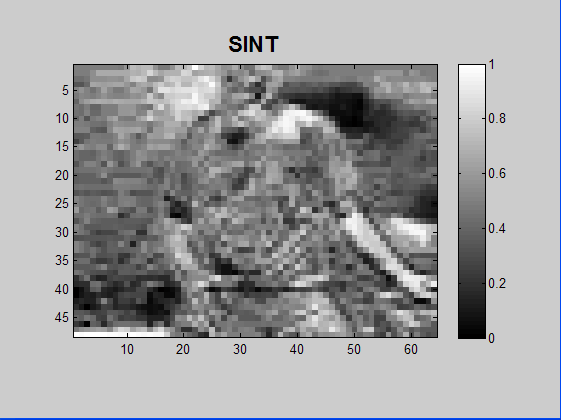
SINT图(垂直方向的微分图):
COST图(水平方向的微分图):

后面3张图看起来有点马赛克效果,那是因为输入的图片最终被缩放到了0.2倍再放大显示的。
实验主要代码及注释
examples.m:
%% EXAMPLES OF IMAGE PROCESSING FOR THE CHALEARN GESTURE CHALLENGE % Isabelle Guyon -- isabelle@clopinet.com -- May 2012 % Most functions work on both [p, n, 3] color images and [p, n] images % Because the RGB channels are identical for depth images, it makes sense % to use only one (but for illustration we work on [p, n, 3] images). % All the functions are independent and can be run on a raw frame, but it % may make sense to chain them. %clear all %close all % close old images if ~exist('this_dir') this_dir=pwd; end data_path = [this_dir '/Examples/']; % Path to the sample data. data_dir = [data_path '/devel/']; % Path to the sample data. code_dir = this_dir; % Path to the code. % Add the path to the function library warning off; addpath(genpath(code_dir)); warning on; %% ================== BEGIN LOADING DATA ====================================== %% == Choose your example == example_num=input('Movie example num [1, 2, or 3]: '); % For each movie, we fetched the labels from train.csv and test.csv if example_num==1 batch_num=1; movie_num=19; train_labels=[10 7 4 2 8 1 6 9 3 5]; test_labels=[10 2 3 3]; elseif example_num==2 batch_num=3; movie_num=16; train_labels=[5 1 4 6 8 7 2 3]; test_labels=[6 2 1 3]; else batch_num=15; movie_num=24; train_labels=[4 3 1 6 5 7 2 8]; test_labels=[4]; end data_name=sprintf('devel%02d', batch_num); %0表示必要时用0来填充,2表示最小显示2位,d表示十进制显示 % Load M and K movies... (fps is the number of frames per seconds) fprintf('Loading movie, please wait...'); [K0, fps]=read_movie([data_dir '/' data_name '_K_' num2str(movie_num) '.avi']); [M0, fps]=read_movie([data_dir '/' data_name '_M_' num2str(movie_num) '.avi']); fprintf(' Done!\n\n'); %% == Image alignment annotations == % Load the alignment information from human annotations for a few frames load([data_path '/image_alignment/image_alignment']); num_frames=length(alignment_labels); % Loads struct alignment_labels and alignment_annotation of dim num_frames % struct alignment_labels { % dataset_name % the batch name % videos % the movie number in the batch % frame } % the frame number in the movie % struct alignment_annotation { % translate_x; % translate_y; % scale_x; % scale_y; } % k_align was selected (by hand) in 1:num_frames to match the videos chosen if example_num==1 k_align=188; elseif example_num==2 k_align=206; else k_align=121; end %strcmp()返回0表示两者不相等,返回1表示两者相等。 if ~strcmp(data_name, alignment_labels(k_align).dataset_name), error('Bad batch name'); end if movie_num~=alignment_labels(k_align).videos, error('Bad movie number'); end % Load average image alignment for an entire batch (these values are % usually pretty good) average=load([data_path '/image_alignment/devel']); %% == Body part annotations == % Load body part annotations from human annotations for a few frames load([data_path '/body_parts/body_parts']); num_frames=length(labels); % Loads struct labels of dim num_frames and the array skeleton_annotation % struct labels { % dataset_name % the batch name % videos % the movie number in the batch % frame } % the frame number in the movie % size(skeleton_annotation) = [num_frames*7, 7] % The columns contain [Frame_ID Body_part_ID Uncertainty x y w h] % where Frame_ID is the line entry is the "labels" struct, Body_part_ID is % 1 : Right hand % 2 : Left hand % 3 : Face % 4 : Right shoulder % 5 : Left shoulder % 6 : Right elbow % 7 : Left elbow % Uncertainty is 0/1 flag indicating if the annotated point is partially visible, % and [x y w h] are the dimensions of the rectangle. % k_body is picked in 1:num_frames to match the videos chosen if example_num==1 k_body=46; %199 elseif example_num==2 k_body=221; else k_body=130; end if ~strcmp(data_name, labels(k_body).dataset_name), error('Bad batch name'); end if movie_num~=labels(k_body).videos, error('Bad movie number'); end %% == Temporal segmentation == % Load temporal segmentation made by humans. % We have the temporal segmentation for all the movie frames of devel01-20 load([data_path '/tempo_segment/' data_name]); % Each Matlab file in segment_dir contains two cell arrays of length 47 % (number of movies): % saved_annotation -- Each element is a matrix (n,2) where n is the number % of gestures in the movie. Each line corresponds to the frame number of % the beginning and end of the gesture. % truth_labels -- Each element is a vector of labels. Normally the % number of labels is equal to n, except if the user % did not perform all the assigned gestures. human_tempo_segment=saved_annotation{movie_num}; truth=truth_labels{movie_num}; %% == Depth normalization coefficients == [MinDepth, MaxDepth]=get_depth_info('Documentation/Depth_info.txt', 'devel', batch_num); %% ======================== END LOADING DATA ==================================== %% ======================== LIST THE CHOICES & CHOOSE ============================= %% == List the choices == choices=list_choices(which('examples')); for k=1:length(choices), fprintf('%2d - %s\n', k, choices{k}); end%输出选择列表 choice=1; e=0; a=-1; while choice ~=0 choice=input('Choice number (or "return" for menu, e or 0 to end, a for all): '); if ~isempty(choice) if choice==-1, choice=1:length(choices); end else choice=-1; end for k=1:length(choice) %length(choice)=1,所以k只能为1? switch choice(k) case -1 %% MENU for k=1:length(choices), fprintf('%2d - %s\n', k, choices{k}); end case 1 %% -- Play movie -- % This uses the image processing toolbox and lauches a movie % player: %implay(M0, fps); % You can also play the depth movie implay(K0); % There is also a simpler movie playing application fprintf(2, ' PLAY MOVIE\nTo play a movie, you can load it with [M, fps]=read_movie(''mymovie.avi'');\nthen run it with play_movie(M0, fps); or implay(M, fps);\n'); play_movie(M0, fps); case 2 %% -- First frame -- fprintf(2, ' FIRST FRAME\nSeveral functions allow you to display images:\nimshow, image, imagesc, imdisplay.\nTo render the depth image in color, use colormap(map);\n'); %Get the first frame in the movie ORIGINAL_K=K0(1).cdata; % Display a frame (grayscale) imdisplay(ORIGINAL_K); % Convert depth to colors (only for depth images, not necessary, just pretty) colormap(jet); % RGB image ORIGINAL_M=M0(1).cdata; imdisplay(ORIGINAL_M); offset_current_figure(100); case 3 %% -- Blurred image -- % Blurr the image (works also for image F(:,:,1) and can be applied several times) % In what follows we don't use blurred images, but this may make sense fprintf(2, ' BLURRED IMAGE\nBlurring is easily achieved with convolutions.\nUse type blurr; to see an example.\n'); ORIGINAL_M=M0(1).cdata; BLURRED_M=blurr(ORIGINAL_M); imdisplay(BLURRED_M); case 4 %% -- Downsized image -- % Rescale an image (native Matlab Image Processing toolbox function) fprintf(2, ' DOWNSIZED IMAGE\nDownsizing is easily achieved with imresize.\n'); scale=0.05; % This means that the image will be reduced to 0.05 time the original size ORIGINAL_M=M0(1).cdata; SMALL_M=imresize(ORIGINAL_M, scale); imdisplay(SMALL_M); case 5 %% -- Gray level image -- % RGB to gray. % Works also for the depth image. However, for the depth image % the 3 channels should be (almost) identical so you can choose % any one of them. So use ORIGINAL_K(:,:,1); fprintf(2, ' GRAY LEVEL IMAGE\nUse rgb2gray to convert a color image to gray levels.\n'); ORIGINAL_M=M0(1).cdata; GRAY_M=rgb2gray(ORIGINAL_M); imdisplay(GRAY_M); case 6 %% -- True depth restoration -- % Restore the original depth values. % Kinect depth images were produced after a normalization f(x)=(x-mini)/(maxi-mini) fprintf(2, ' TRUE DEPTH RESTORATION\nThe data were rescaled between 1 and 255.\nTo get the original values, read the normalization coefficients from\nDocumentation/Depth_info.txt\nand use the formula RESTORED_K=GRAY_K/255*(MaxDepth-MinDepth)+MinDepth;\n'); ORIGINAL_K=K0(1).cdata; GRAY_K=double(ORIGINAL_K(:,:,1)); Diff=MaxDepth-MinDepth; RESTORED_K=GRAY_K/255*Diff+MinDepth; imdisplay(RESTORED_K); case 7 %% -- Background removal -- % For depth images only! This will give odd results on color images % Remove the image background (works also for image F(:,:,1)) fprintf(2, ' BACKGROUND REMOVAL\nUse bgremove(image) to take out the background of depth images\nor clean_movie(K) to apply it to an entire movie K.\n'); ORIGINAL=K0(1).cdata; NO_BACKGROUND=bgremove(ORIGINAL); imdisplay(NO_BACKGROUND); % You can use the following function to clean the whole movie clean_all=input('Do you want to clean the whole movie [y/n]? ', 's'); if strcmp(clean_all, 'y') fprintf('Wait, cleaning...\n'); M=clean_movie(K0); play_movie(M); set(gcf, 'Name', 'CLEAN MOVIE'); end case 8 %% -- Head detection -- % In depth images with no occlusion. % This calls inside bgremove. fprintf(2, ' HEAD DETECTION\nFor various normalizations it is often useful to locate the head.\nUse detect_head(frame1, frame2) to locate the head in the first frame.\n'); if example_num~=2 ORIGINAL=K0(1).cdata; imdisplay(ORIGINAL, figure, 'HEAD BOX'); hold on % Uses two consecutive frames SECOND=K0(2).cdata; head_box=detect_head(ORIGINAL, SECOND); rectangle('Position', head_box, 'EdgeColor', 'b', 'Linewidth', 2); else fprintf('Works only in depth images without occlusions.\n'); end case 9 %% -- Manual body part annotations -- % Show the annotations made by humans fprintf(2, ' MANUAL BODY PART ANNOTATIONS\nA subset of the frames were MANUALLY annotated.\nThe annotations are found in Examples/body_parts.mat.\nThe documentation is found in Documents/README_BODY_PARTS.txt.\n'); frame_num=labels(k_body).frame; IMAGE_K=K0(frame_num).cdata; annot=skeleton_annotation(skeleton_annotation(:,1)==k_body,2:end); display_annot(IMAGE_K, annot, figure, 'BODY PART ANNOTATIONS (man-made)'); case 10 %% -- Automatic body part annotations -- % Head, hand and shoulder detection, from a single depth frame % For depth images only. This works well only if the face is detected well % (not in example 2 where the head is occluded). fprintf(2, ' AUTOMATIC BODY PART ANNOTATIONS\nWe provide a set of functions (detect_head, detect_hand, detect_shoulder)\nto automatically detect body parts.\n'); if example_num~=2 fprintf('A little slow, be patient...\n'); ORIGINAL_K=K0(1).cdata; frame_num=labels(k_body).frame; IMAGE_K=K0(frame_num).cdata; imdisplay(IMAGE_K, figure, 'BODY PART ANNOTATIONS (automatic)'); hold on % Face from a single frame face_box=detect_head(IMAGE_K); rectangle('Position', face_box, 'EdgeColor', 'b', 'Linewidth', 2); % (Single) hand detection on depth image % For faster usage, the face position can be passed as an argument [~, ~, hand_box] = detect_hand(IMAGE_K, ORIGINAL_K); rectangle('Position', hand_box, 'EdgeColor', 'g', 'Linewidth', 2); % Shoulder detection on depth image [~, ~, ~, left_box, right_box] = detect_shoulder(IMAGE_K); rectangle('Position', left_box, 'EdgeColor', 'm', 'Linewidth', 2); rectangle('Position', right_box, 'EdgeColor', 'y', 'Linewidth', 2); else fprintf('==> Sorry, not available for this example:\n It works only in depth images without occlusions.\n\n'); end case 11 %% -- Body segmentation -- % Slower function for depth images only to isolate the body on depth images. % We choose the frame for which we know the human annotations fprintf(2, ' BODY SEGMENTATION\nThe function detect_body_segment separates the body from the background\non depth images. It is slower than bgremove, but does a better job.\n'); frame_num=alignment_labels(k_align).frame; IMAGE_K=K0(frame_num).cdata; BODY_SEGMENTATION = detect_body_segment(IMAGE_K); imdisplay(BODY_SEGMENTATION); case 12 %% -- Manual alignment depth/RGB -- fprintf(2, ' MANUAL ALIGNMENT DEPTH/RGB\nA subset of the frames were MANUALLY aligned.\nThe alignment is found in Examples/image_alignment.\nThe documentation is found in Documents/README_IMAGE_ALIGNMENT.txt and Documents/LOOK_AT_ME.jpg.\nWithin a batch, the average alignment parameters can be used.\n'); % We suggest to use average alignment parameters for the whole batch average_alignment=1; % The original images are not well aligned. frame_num=alignment_labels(k_align).frame; IMAGE_K=K0(frame_num).cdata; IMAGE_M=M0(frame_num).cdata; BODY_SEGMENTATION = detect_body_segment(IMAGE_K); for k=1:3 I=IMAGE_M(:,:,k); if k==3, I(BODY_SEGMENTATION==0)=120; else, I(BODY_SEGMENTATION==0)=0; end OVERLAID_IMAGES(:,:,k)=I; end imdisplay(OVERLAID_IMAGES); % We do not have yet a good alignment algorithm, but we provide image % annotations for a few image frames if average_alignment annot=average.alignment_annotation(batch_num); else annot=alignment_annotation(k_align); end ALIGNED_IMAGES = apply_alignment(IMAGE_M, IMAGE_K, ... annot.translate_x, annot.translate_y, annot.scale_x, annot.scale_y); imdisplay(ALIGNED_IMAGES); offset_current_figure(100); case 13 %% -- Approximated gradients -- % Works both for RGB and depth, we show RGB. % Compute approximate gradients (works also for image F(:,:,1)) % It works on the original image too, we show here an examples after % removing the background. fprintf(2, ' APPROXIMATED GRADIENTS\nTo approximate gradients, we compute differences between the image and a shifted version to the right or down. We then get the norm and by normalizing, the sine and cosine. See approx_grad for more details.\n'); scale=0.2; % This means that the image will be reduced to 0.2 time the original size isd=0; % change to isd=1 to see the depth image case if isd IMAGE=bgremove(rgb2gray(K0(1).cdata));%如果是深度图像的话则这里显示的是去除背景后的图像 else IMAGE=rgb2gray(M0(1).cdata); end M0(1) [p, n, d]=size(IMAGE) imshow(IMAGE) [RHO, SINT, COST] = approx_grad(IMAGE, scale); imdisplay(RHO); % This is the norm of the direction vector imdisplay(SINT); % This is its sine offset_current_figure(100);%为了不重叠显示这些图片,平移一下 imdisplay(COST); % This is its cosine offset_current_figure(200); % This slow function shows the gradients as little oriented arrows display_arrows=input('Do you want to see the gradients as little arrows (slow) [y/n]? ', 's'); if strcmp(display_arrows, 'y') fprintf('A little slow, be patient...\n'); show_grad(RHO, SINT, COST); end case 14 %% -- Image differences -- % Works both of RGB and depth, we show depth. % Differences between images are informative % Be carefull, if you don't convert to double, the negative values will be % clipped (see whether this is what you want) fprintf(2, ' IMAGE DIFFERENCES\nSimple consecutive image differences carry a lot of information. If you do differences of uint8 images, only the positive part it kept, see whether this is what you want.\n'); isd=1; % change to isd=0 to see the RGB image if isd SIXTH=bgremove(K0(6).cdata); FIFTH=bgremove(K0(5).cdata); else SIXTH=M0(6).cdata; FIFTH=M0(5).cdata; end DIFFERENCE=SIXTH-FIFTH; imdisplay(FIFTH); imdisplay(SIXTH); offset_current_figure(100); imdisplay(DIFFERENCE); offset_current_figure(200); case 15 %% -- Motion energy histograms -- % Works both of RGB and depth, we show depth. % This function converts the entire movie into a data matrix % with dimension [nf, dc] where nf is the number of frames -1 and dc the % number of pixels in the image after rescaling. % It uses differences in the R channel only. % This function is used in the @principal_motion recognizer example fprintf(2, ' MOTION ENERGY HISTOGRAMS\nWe can create a useful representation by averaging frame differences in a coarse image grid, see motion_histograms.\n'); scale=0.2; isd=1; % change to isd=0 to see the RGB image if isd M=K0; else M=K; end [MOTION_HISTOGRAMS, p, n]=motion_histograms(M, scale); imdisplay(MOTION_HISTOGRAMS'); axis normal xlabel('Time', 'Fontsize', 14, 'Fontweight', 'bold'); ylabel('Motion histogram features', 'Fontsize', 14, 'Fontweight', 'bold'); set(gcf, 'Name', 'MOTION_HISTOGRAMS FEATURES'); case 16 %% -- Principal components -- % Computed on depth motion histograms, works for RGB too. % If is often useful to reduce the representation to its principal components % Here we show a reduction of the motion histograms to 9 principal components % This function is used in the @principal_motion recognizer example fprintf(2, ' PRINCIPAL COMPONENTS\nWe apply principal component analysis to motion energy histograms. We show the 9 first principal components.\n'); scale=0.2; isd=1; % change to isd=0 to see the RGB image if isd M=K0; else M=K; end [MOTION_HISTOGRAMS, p, n]=motion_histograms(M, scale); % Compute PC pcs=9; PC = pc_compute( MOTION_HISTOGRAMS, pcs ); % Project the representation on the principal component subspace nf=size(MOTION_HISTOGRAMS, 1); MOTION_PCA=MOTION_HISTOGRAMS-PC.mu(ones(nf,1),:); % center MOTION_PCA=MOTION_PCA*PC.U; imdisplay(MOTION_PCA'); axis normal xlabel('Time', 'Fontsize', 14, 'Fontweight', 'bold'); ylabel('PCA features', 'Fontsize', 14, 'Fontweight', 'bold'); set(gcf, 'Name', 'PRINCIPAL COMPONENT FEATURES'); % Show the principal components (principal motions) dim=sqrt(pcs); h=figure; for j=1:pcs subplot(dim, dim, j); im=PC.U(:,j); im=reshape(im, p, n); imdisplay(im, h, ['PC ' num2str(j)]); axis off end set(gcf, 'Name', 'PRINCIPAL COMPONENTS'); %% -- Flow -- % Gradient on image difference: some kind of flow (not great) %[RHOF, SINTF, COSTF] = approx_grad(DIFFERENCE, scale); %imdisplay(RHOF); %imdisplay(SINTF); %imdisplay(COSTF); %% -- Active motion -- % Works both of RGB and depth, we show RGB. % Because motion seems so important, we wrote this function that seems to % do a good job at filtering motion. It uses as first argument the image of % interest and as other arguments the previous, next and original frames. % You may only provide a subset of those if you want. % Here we work without background, see whether this makes sense for you. % Note: This is not optimized for speed. % But this is not really better than just differences, so we % took it out... if 1==2 isd=0; % change to isd=1 to see the depth image if isd NO_BACKGROUND=bgremove(K0(1).cdata); SIXTH=bgremove(K0(6).cdata); FIFTH=bgremove(K0(5).cdata); SEVENTH=bgremove(K0(7).cdata); else NO_BACKGROUND=M0(1).cdata; SIXTH=M0(6).cdata; FIFTH=M0(5).cdata; SEVENTH=M0(7).cdata; end ACTIVE_MOTION = active_motion(SIXTH, FIFTH, SEVENTH, NO_BACKGROUND); imdisplay(ACTIVE_MOTION); end case 17 %% -- Motion history -- % Works both of RGB and depth, we show RGB fprintf(2, ' MOTION HISTORY\nWe use differences between consecutive frames to track motion in a function called motion_trail. We show the average (motion average) and stacked images with an index varying in time (motion history).\n'); isd=1; % change to isd=0 to see the RGB image if isd M=K0; else M=M0; end % We can get a motion trail for the whole movie fprintf('A little slow, be patient...\n'); [MOTION, MOTION_AVERAGE, MOTION_HISTORY] = motion_trail(M); MOTION_AVERAGE=log(1+MOTION_AVERAGE); imdisplay(MOTION_AVERAGE); % Take log to increase contrast imdisplay(MOTION_HISTORY); offset_current_figure(100); colormap(jet); show_movie=input('Do you want to see the motion energy movie [y/n]? ', 's'); if strcmp(show_movie, 'y') play_movie(MOTION); end case 18 %% -- Static posture history -- %Works both of RGB and depth, we show depth. fprintf(2, ' STATIC POSTURE HISTORY\nWe use differences between consecutive frames and with the original frame to detect static postures with the function motion_trail. We show the average (static average) and stacked images with an index varying in time (static history).\n'); isd=1; % change to isd=0 to see the RGB image if isd M=K0; else M=M0; end static=1; [STATIC, STATIC_AVERAGE, STATIC_HISTORY] = motion_trail(M, static); STATIC_AVERAGE=log(1+STATIC_AVERAGE); % Take log to increase contrast imdisplay(STATIC_AVERAGE); imdisplay(STATIC_HISTORY); offset_current_figure(100); colormap(jet); show_movie=input('Do you want to see the movie of "static" postures [y/n]? ', 's'); if strcmp(show_movie, 'y') play_movie(STATIC); end case 19 %% -- HOG and HOF -- % Works both of RGB and depth, we show RGB. % From Piotr's Image and Video Matlab Toolbox (PMT) % http://vision.ucsd.edu/~pdollar/toolbox/doc/index.html % Requires the image processing toolbox fprintf(2, ' HOG AND HOF\nHistograms of Oriented Gradients (HOG) and Histograms of Optical Flow (HOF) can be computed with Piotr''s Image and Video Matlab Toolbox (PMT), redistributed with this package. Other useful functions may be found in that package.\n'); isd=0; % change to isd=1 to see the depth image if isd SIXTH=bgremove(K0(6).cdata); FIFTH=bgremove(K0(5).cdata); else SIXTH=M0(6).cdata; FIFTH=M0(5).cdata; end % HOG F1=double(FIFTH); % Must convert to double Fhog=hog(F1,8,9); % spacial bin size=8, num orientation bins=9 % Show the HOG features HOG=hogDraw(Fhog,25); imdisplay(HOG); % fold 4 normalizations nFold=4; s=size(Fhog); s(3)=s(3)/nFold; w0=Fhog; Fhog=zeros(s); for o=0:nFold-1, Fhog=Fhog+w0(:,:,(1:s(3))+o*s(3)); end; % Optical flow (needs two 2d images, generally consecutive) F2=double(SIXTH); I1=F1(:,:,1); I2=F2(:,:,1); h=figure; [Vx,Vy,reliab] = optFlowLk( I1, I2, [], 4, 1.2, 3e-6, h ); title('OPTICAL FLOW'); set(h, 'Name', 'OPTICAL FLOW'); offset_current_figure(100); case 20 %% -- Human temporal segmentation -- % From human annotations, diplayed with truth values on motion % trail of depth image. % We can use the active motion to temporally segment fprintf(2, ' HUMAN TEMPORAL SEGMENTATION\nAll the videos in devel01-20 were MANUALLY segmented into isolated gestures.\nThe annotations are found in Examples/tempo_segment.\nThe documentation is found in Documents/README_TEMPO_SEGMENT.txt.\n'); isd=0; % change to isd=1 to see the depth image if isd M=K0; else M=M0; end % We can get a motion trail for the whole movie %static=0; %[~,~,~, MOTION_TRAIL] = motion_trail(M, static); MOTION_TRAIL=motion(M); % This is faster and the slower one does not really get more intersting results display_segment(MOTION_TRAIL, human_tempo_segment, truth); set(gcf, 'Name', 'HUMAN TEMPORAL SEGMENTATION'); case 21 %% -- Dynamic Time Warping (DTW) recognition-based segmentation -- % This example show how recognition and temporal segmentation % can be performed with Dynamic Time Warping. % We use the depth image only here but this works with RGB too. % We compute simple motion features and use them for temporal % segmentation and recognition. The temporal segmentation is % generally correct, even when the gesture recognition is % incorrect. % There are 2 variants, with an without returning to the rest % position. with_rest_position=0; fprintf(2, ' DYNAMIC TIME WARPING (DTW) RECOGNITION-BASED SEGMENTATION\nIn this example, we use the motion average in 9 parts of the image as a function of time. We perform DTW between the training examples and the test video. The best path alows us to find the temporal segmentation.\nWe show the motion feature representation at the top and at the bottom, the class labels in the segments on top of the maximum motion as a function of time. Using a few motion features usually gives a good segmentation but may give poor recognition.\n'); if with_rest_position fprintf(2, 'We force the model to return to the resting position in between gestures. The label for the rest position is 1+num_classes\n'); end % TRAINING DATA fprintf('Loading training data...'); n=length(train_labels); for k=1:n Ktr{k}=read_movie([data_dir data_name '_K_' num2str(k) '.avi']); end fprintf(' done\n'); % DTW RECOGNITION-BASED SEGMENTATION [auto_tempo_segment, MOTION_te, recognized_labels]=dtw_example(Ktr, train_labels, K0, with_rest_position); % Simple temporal sequence used for display purpose motion_score=max(MOTION_te,[],2); % Show the results, with comparison with human segmentation h=figure; hold on subplot(3,1,1); imdisplay(MOTION_te', h, 'MOTION FEATURES'); axis normal; colorbar off subplot(3,1,2); display_segment(motion_score, auto_tempo_segment, recognized_labels, h); title('Automatic segmentation', 'Fontsize', 16, 'FontWeight', 'bold'); subplot(3,1,3); display_segment(motion_score, human_tempo_segment, truth, h); title('Human segmentation', 'Fontsize', 16, 'FontWeight', 'bold'); offset_current_figure(100); set(gcf, 'Name', 'DYNAMIC TIME WARPING (DTW) TEMPORAL SEGMENTATION'); case 22 %% -- Hand-motion temporal segmentation (NO DTW) -- % Temporal segmentation of a video based on motion, % without using dynamic time warping. The method can be used in on-line % mode, ie without waiting for the end of the video. % No training examples are needed. % Both RGB and depth images are used. % Since the code relies on hands detector and face detector, % it won't work well for batches where you can't see the whole head. % For example, example no.2 in the sample files. fprintf(2, ' HAND-MOTION TEMPORAL SEGMENTATION\nIn this example, temporal segmentation is performed without training examples and DTW, just using the hand motion.\n'); if example_num==2, fprintf('Warning: Does not work well is the head is occluded.\n\n'); end [auto_tempo_segment, motion_score] = temporal_segment(K0, M0); % Show the results, with comparison with human segmentation h=figure; hold on subplot(2,1,1); display_segment(motion_score, auto_tempo_segment, [], h); title('Automatic segmentation', 'Fontsize', 16, 'FontWeight', 'bold'); subplot(2,1,2); display_segment(motion_score, human_tempo_segment, truth, h); title('Human segmentation', 'Fontsize', 16, 'FontWeight', 'bold'); offset_current_figure(100); set(gcf, 'Name', 'HAND-MOTION TEMPORAL SEGMENTATION'); % Another way to display predictions overlaying automatic and % human segmentation. %plot_prediction(auto_tempo_segment, human_tempo_segment, motion_trail); case 23 %% -- Extract skeleton w. ETH code -- % Works both of RGB and depth, we show depth. It works poorly % for gestures where body parts lie withing the torso area and % when the user is too close to the sensor. It uses the pose % estimation code by Marcin Eichner, Manuel J. Mar韓-Jim閚ez, % Andrew Zisserman, and Vittorio Ferrari, available from % http://www.vision.ee.ethz.ch/~calvin/articulated_human_pose_estimation_code/ % To extract the skeleton from another video you will have to % install the afore mentioned pose estimation code % Add the pose estimation code to the path: % addpath(genpath('../Path to pose estimation code/..')); % Load precalculated parameters for the model: % load env.mat % Extract skeleton % [skeleton_annotation_pred] = get_skeleton_from_vid(K0, ... % fghigh_params,parse_params_Buffy3and4andPascal,pm2segms_params); % Load precalculated body parts and display the result (a matrix skeleton_annotation_pred) fprintf(2, ' EXTRACT SKELETON W. ETH CODE\nThis is a pre-recorded example of skeleton extraction. The code of Marcin Eichner, Manuel J. Mar韓-Jim閚ez, Andrew Zisserman, and Vittorio Ferrari is available from http://www.vision.ee.ethz.ch/~calvin/articulated_human_pose_estimation_code/\n'); isd=1; if isd, movie_type='K'; M=K0; else movie_type='M'; M=M0; end s=load(['skeleton_data_ETH_' num2str(batch_num) '_' movie_type '_' num2str(movie_num)]); if example_num==1 % The method works pretty well for the first example frame_num=15; elseif example_num==2 % It mostly fails for the second one fprintf('==> Sorry, this code does not work well with occluded images.\n\n'); frame_num=139; else % The method works OK for the third example frame_num=29; end display_skeleton_data(M,s.skeleton_annotation, frame_num); % Process the entire movie and get the time series for % Head, Torso, upper right and left arm and lower right and % left arm (6 time series), remove the last argument and run all_frames=input('Do you want to process the whole movie [y/n]? ', 's'); if strcmp(all_frames, 'y') M=display_skeleton_data(M,s.skeleton_annotation); replay=input('Do you want to replay the movie [y/n]? ', 's'); if strcmp(replay, 'y') implay(M, fps); end end case 24 %% -- Find body parts w. D. Ramanan s code -- % Works both of RGB and depth, we show depth. It uses the pose % estimation code by Deva Ramanan % the code is publicly available from % http://www.vision.ee.ethz.ch/~calvin/articulated_human_pose_estimation_code/ % % To extract the skeleton from another video you will have to % install the afore mentioned pose estimation code % Extract skeleton % [BSX] = extract_DR_boxes(V0); % Load precalculated body parts and display the result % % Note: this code does not work great on these data, it % probably needs retraining for the kind of images we are % dealing with. fprintf(2, ' FIND BODY PARTS W. D. RAMANANS CODE\nThis is a pre-recorded example of body part extraction. The code of Deva Ramanan is available from http://phoenix.ics.uci.edu/software/pose/\n'); % Works both for depth and RGB images, we show RGB isd=0; if isd, movie_type='K'; M=K0; frame_num=8; %Cherry picked by hand else movie_type='M'; M=M0; frame_num=15; %Cherry picked by hand end if example_num==1, fprintf('==> Sorry, this code does not work well with a busy background.\n\n'); elseif example_num==2 fprintf('==> Sorry, this code does not work well with occluded images.\n\n'); else load(['skeleton_data_Deva_' num2str(batch_num) '_' movie_type '_' num2str(movie_num)]); display_boxes_Deva(M, BSX, frame_num); all_frames=input('Do you want to process the whole movie [y/n]? ', 's'); if strcmp(all_frames, 'y') M=display_boxes_Deva(M, BSX); replay=input('Do you want to replay the movie [y/n]? ', 's'); if strcmp(replay, 'y') implay(M, fps); end end end case 25 %% -- STIP features -- % We are making the gesture challenge data available as pre-computed STIP features % (http://www.irisa.fr/vista/Equipe/People/Laptev/download.html#stip). % The STIP code is available for free use for research and development activities, % including entering the gesture challenge and competing for prizes. % If you use these features and publish your work, please give credit to the authors % by citing their papers [Laptev, IJCV 2005], [Laptev et al. CVPR 2008]. % For product commercialization, including licensing code to Microsoft, please contact % Ivan Laptev at INRIA http://www.di.ens.fr/~laptev. % We also use: % http://www.di.ens.fr/willow/events/cvml2010/materials/practical-laptev/. fprintf(2, ' STIP FEATURES\nWe are making the gesture challenge data available as pre-computed STIP features (http://www.irisa.fr/vista/Equipe/People/Laptev/download.html#stip). The STIP code is available for free use for research and development activities, including entering the gesture challenge and competing for prizes. If you use these features and publish your work, please give credit to the authors by citing their papers [Laptev, IJCV 2005], [Laptev et al. CVPR 2008]. For product commercialization, including licensing code to Microsoft, please contact Ivan Laptev at INRIA http://www.di.ens.fr/~laptev.\n'); % This works both with RGB and depth movies, we show the depth movies isd=0; if isd, movie_type='K'; M=K0; else movie_type='M'; M=M0; end % Cherry picked frames if example_num==1 if isd, frame_num=46; else frame_num=93; end elseif example_num==2 frame_num=69; else frame_num=19; end % Read the STIP features % pos: point-type y x t sigma2 tau2 % val: detector-confidence % descr: dscr-hog(72) dscr-hof(90) [pos, val, dscr]=readstips_text([data_path '/STIP/' data_name '_' movie_type '_' num2str(movie_num) '.txt']); % Show the circles with the STIP features locations show_circle_stip(M, pos, 1, 0, frame_num); set(gcf, 'Name', 'STIP FEATURES'); % Process the whole movie all_frames=input('Do you want to process the whole movie [y/n]? ', 's'); if strcmp(all_frames, 'y') MS=show_circle_stip(M, pos); replay=input('Do you want to replay the movie [y/n]? ', 's'); if strcmp(replay, 'y') implay(MS, fps); end end case 26 %% -- Bag of STIP features -- % We use the STIP features of case 25 and follow % http://www.di.ens.fr/willow/events/cvml2010/materials/practical-laptev/ % to compute the STIP features. fprintf(2, ' BAG OF STIP FEATURES\nWe cluster the STIP features in training data. The cluster centers represent meta-features. We represent video sequences as a histogram of presence of such meta-features. The position information of the STIP features is not used.\n'); % This works both with RGB and depth movies, we show the depth movies isd=1; if isd, movie_type='K'; M=K0; else movie_type='M'; M=M0; end n_tr=length(train_labels); % Number of training examples train_data=[data_path '/STIP/' data_name '_' movie_type '_']; % Base of the STIP feature file names % one then appends [num_movie].txt to get the % STIP filename test_data=[data_path '/STIP/' data_name '_' movie_type '_' num2str(movie_num) '.txt']; % Test STIP filename cnum=30; % Number of cluters rep=1; % Choice of representation (subset of features) nover=3; % Sliding window overlap % Get STIP feature cluster centers and BOF representation for % training data [BOF_tr, centers, tr_duration] = train_STIP_BOF(train_data, n_tr, cnum, rep); % Get STIP BOF representation of test data in a sliding window, [BOF_te, FEAT_te, POS_te] = sliding_STIP_BOF(test_data, centers, tr_duration, rep, nover); % Compute the distance between the meta-frames and the % templates (training examples) [s, idx]=sort(train_labels); DISTANCE_TO_TEMPLATES=eucliddist(BOF_tr(idx, :), BOF_te); imdisplay(DISTANCE_TO_TEMPLATES); xlabel(['True labels: ', sprintf('%d ', test_labels)], 'FontSize', 16, 'FontWeight', 'bold'); % Visualization of features labeled by cluster centers (pretty, % not very useful) all_frames=input('Do you want to see the feature positions on the movie [y/n]? ', 's'); if strcmp(all_frames, 'y'); dist=eucliddist(centers, FEAT_te); [sdist, lbl]=min(dist); fprintf(2, 'The different colors represent the cluster centers\n'); MC=show_circle_stip(M, POS_te, lbl); set(gcf, 'Name', 'STIP FEATURES CLUSTERS'); replay=input('Do you want to replay the movie [y/n]? ', 's'); if strcmp(replay, 'y') implay(MC, fps); end end otherwise %fprintf('No such choice\n'); end end end
approx._grad.m(计算梯度的核心函数):
function [RHO, SINT, COST] = approx_grad( M , scale, debug )
%[RHO, SINT, COST] = approx_grad( M , scale, debug )
% Compute the norm RHO and the cosine and sine SINT and COST of the
% gradients at evey pixel in image M in an approximate way.
% M -- image (gray scale)
% scale -- factor by which to rescale the image (rescaling a the end, not
% faster)
% debug -- 1 to show images

% Isabelle Guyon -- isabelle@clopinet.com -- April 2012

if nargin<2, scale=1; end
if nargin<3, debug=0; end

if ~isa(M, 'double'), M=double(M); end

[p, n, d]=size(M);%本例中,p=240,n=320,d=1;p为高度,n为宽度
% Vertical differences,垂直方向上的差分,每个像素点的垂直差分上它下面的点减去去上面的点
SINT=M(3:p, 1:n, :)-M(1:p-2, 1:n, :); SINT=[SINT(1,:, :); SINT; SINT(end,:, :)];
% Horizontal differences
COST=M(1:p, 3:n, :)-M(1:p, 1:n-2, :); COST=[COST(:,1, :), COST, COST(:,end, :)];
% Norm
RHO=sqrt(SINT.^2+COST.^2);

if nargout>1
    NORMA=RHO;
    NORMA(RHO==0)=eps;%eps为1的精度,用很小的数代替幅值0
    % Normalization (we take the perpendicular to be consistent with other work)
    SINT=SINT./NORMA;
    COST=COST./NORMA;
end

if scale<1 && scale>0
    miniM=imresize(M, scale); % better to reduce first for the norm
    RHO=approx_grad(miniM);
    if nargout>1 % better the compute the direction before reducing
        SINT=imresize(SINT, scale);%SINT和COST是计算完后再缩放,而不是先缩放再计算
        COST=imresize(COST, scale);
    end
end

if debug>0
    imdisplay(RHO);
    imdisplay(SINT);
    imdisplay(COST);
end

end
imdisplay(显示图片的函数):
function h = imdisplay( im, h, ttl )
%h = imdisplay( im, h, ttl )
% Display grayscale images.

% Isabelle Guyon -- isabelle@clopinet.com -- April 2012

if nargin<3
    ttl=inputname(1);
    ttl(ttl=='_')=' ';
end
if nargin<2, h=figure; else figure(h); end %h是个句柄号
set(h, 'Name', ttl);

[ISKINECT, im]=is_depth(im);

if isa(im, 'double')
    mini=min(im(:));
    maxi=max(im(:));
    im=(im-mini)./(maxi-mini);
end
imagesc(im); %类似于imshow,只不过它是把矩阵当做图片显示出来
axis image

if ISKINECT
    colormap(gray);
    colorbar;
end


title(ttl, 'Fontsize', 16, 'FontWeight', 'bold');
实验总结
如果掌握了matlab一些常用的交互设计的话,那么很多程序编写起来就方便不少。梯度图一般指的是幅值图,即水平梯度图(右边减掉坐标)和垂直梯度图(左边减掉右边)的合成,马赛克是由于图片进行梯度计算前缩小了,计算完后又放大了的缘故。
参考资料
ChaLearn Gesture Challenge_2:examples体验
http://gesture.chalearn.org/data/sample-code

 浙公网安备 33010602011771号