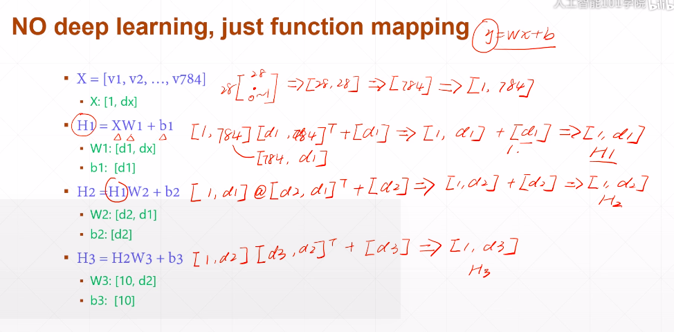
手写数字问题

 

 

H3:[1,1] #第一个1表示照片数量，第二个1表示0～9的一个数字
one-hot(上图)就没有1<2<3的大小关系了 #编码方式

 

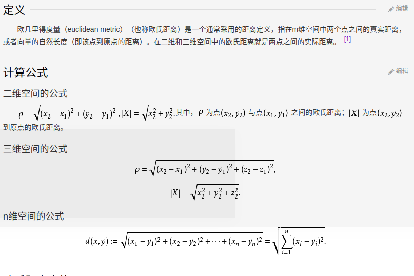
欧式距离

 

 

 

 

 

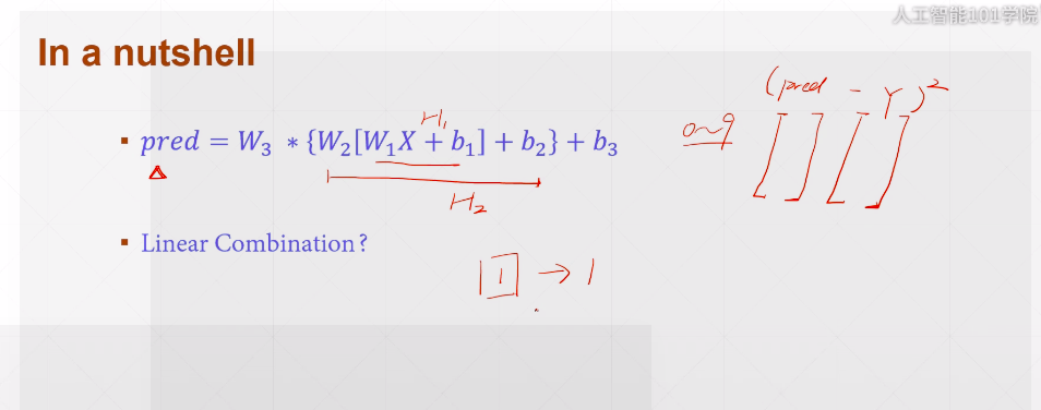
线性很难识别现实的数字问题，如1的字体、倾斜度等

 

 

 

 

 

 

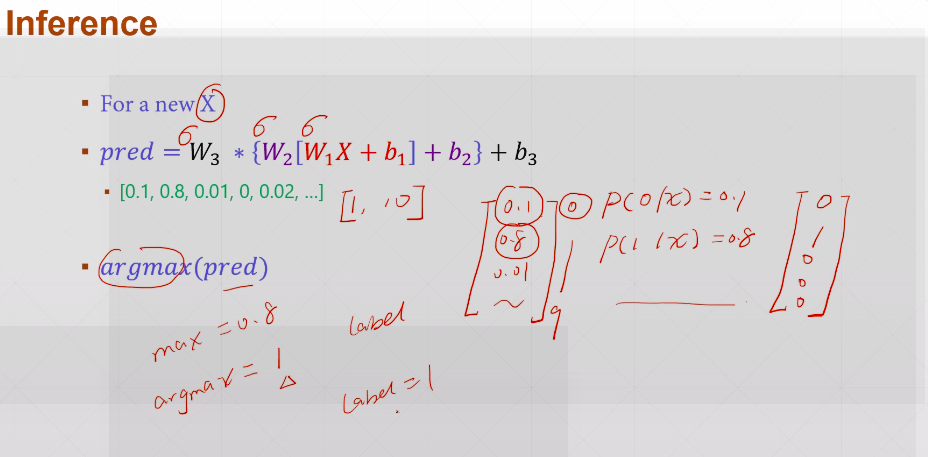
P(1|x)=0.8  #给定x ，label(也就是y)为1的概率为0.8
argmax(pred)  #pred在的索引号

 

'''
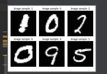
utils.py

'''
import torch
from matplotlib import pyplot as plt
def plot_curve(data):
    fig = plt.figure()
    plt.plot(range(len(data)), data, color='blue')
    plt.legend(['value'], loc='upper right')
    plt.xlabel('step')
    plt.ylabel('value')
    plt.show()


def plot_image(img, label, name):

    fig = plt.figure()
    for i in range(6):
        plt.subplot(2, 3, i+1)
        plt.tight_layout()
        plt.imshow(img[i, 0]*0.3081+0.1307, cmap='gray', interpolation='none')
        plt.title("{}: {}".format(name,label[i].item()))
        plt.xticks([])
        plt.yticks([])
    plt.show()

def one_hot(label, depth=10):
    out = torch.zeros(label.size(0), depth)
    idx = torch.LongTensor(label).view(-1, 1)
    out.scatter_(dim=1, index=idx, value=1)
    return out

 

 

import torch
from torch import nn
from torch.nn import functional as F

from    torch import optim#不加后面的optimizer = optim.SGD(net.parameters(), lr=0.01, momentum=0.9)会报错

import torchvision
from matplotlib import pyplot as plt
from utils import plot_image, plot_curve, one_hot
#from utils import plot_image, plot_curve, one_hot
batch_size = 512 #一次处理图片的数量
train_loader = torch.utils.data.DataLoader(
    #download = True  当前没有mnist_data时，会自动从网上下载
    #Normalize 正则化:使数据在0附近均匀分布，会提升性能到80%
    torchvision.datasets.MNIST('mnist_data', train=True, download=True,
                               transform=torchvision.transforms.Compose([
                                   torchvision.transforms.ToTensor(),
                                   torchvision.transforms.Normalize(
                                       (0.1307,), (0.3081,))
                               ])),
    batch_size=batch_size, shuffle=True)
test_loader = torch.utils.data.DataLoader(
    torchvision.datasets.MNIST('mnist_data/', train=False, download=True,
                               transform=torchvision.transforms.Compose([
                                   torchvision.transforms.ToTensor(),
                                   torchvision.transforms.Normalize(
                                       (0.1307,), (0.3081,))
                               ])),
    batch_size=batch_size, shuffle=False)
x, y = next(iter(train_loader))
print(x.shape, y.shape, x.min(), x.max())
#plot_image(x, y, 'image sample')

 

 

 

 

 

 

 

 

 

plot_image(x, y, 'image sample')

 

 

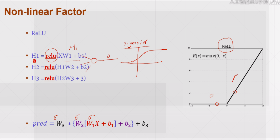
# step2 build network three layers

class Net(nn.Module):
    def __init__(self):
        super(Net, self).__init__()

        # xw+b
        '''
        28×28,256 #256是按经验得到的
        256，64#上层的输出是下层的输入
        64,10#10个输出节点0～9：10分类
        '''
        self.fc1 = nn.Linear(28*28, 256)
        self.fc2 = nn.Linear(256, 64)
        self.fc3 = nn.Linear(64, 10)

    def forward(self, x):
        # x:[b,1,28,28]
        #h1 = relu(xw1+b1)
        x = F.relu(self.fc1(x))
        #h2 = relu(h1w2+b2)
        x = F.relu(self.fc2(x))
        # h3 = (h2w3+b3)
        x = self.fc3(x)
        return x

 

#step3 :  Train
net  =Net()#顶格才可以
optimizer = optim.SGD(net.parameters(), lr=0.01, momentum=0.9)

train_loss = []

for epoch in range(3): #for必须顶格

     for batch_idx, (x,y) in enumerate(train_loader):
         #x : [b,1,28,28] ,y :[512]
         #[b, 1, 28, 28] => [b,feature]
         x = x.view(x.size(0), 28*28) #[b,784]
         #=> [b,10]
         out = net(x)
         # [b,10]
         y_onehot = one_hot(y)
         loss = F.mse_loss(out, y_onehot)#out, y_onehot的均方差
         optimizer.zero_grad()#清零梯度
         loss.backward() #loss.backward() 计算梯度
         # w' = w -lr*grad
         optimizer.step()#更新梯度

         train_loss.append(loss.item())

if batch_idx % 10 ==0:
             print(epoch, batch_idx, loss.item())

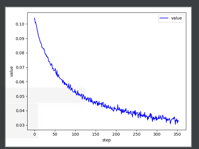
plot_curve(train_loss)#更加形象的表示下降过程，顶格不要进入for的范围

# we get optimal [w1,b1,w2,b2,w3,b3]

/usr/bin/python3.5 /home/chenliang/PycharmProjects/train1/train.py
0 0 0.10039202123880386
0 10 0.09092054516077042
0 20 0.08298195153474808
0 30 0.07697424292564392
0 40 0.07104992121458054
0 50 0.06729131937026978
0 60 0.06352756172418594
0 70 0.059826698154211044
0 80 0.05679488927125931
0 90 0.05659547820687294
0 100 0.0517868809401989
0 110 0.05031196400523186
1 0 0.05097236484289169
1 10 0.045329973101615906
1 20 0.04571853205561638
1 30 0.04453044757246971
1 40 0.040699463337659836
1 50 0.041865888983011246
1 60 0.0409906730055809
1 70 0.04103473946452141
1 80 0.04012298583984375
1 90 0.040163252502679825
1 100 0.039349883794784546
1 110 0.03824656829237938
2 0 0.03849620744585991
2 10 0.037528540939092636
2 20 0.036403607577085495
2 30 0.034915562719106674
2 40 0.036890819668769836
2 50 0.03506477177143097
2 60 0.03299033269286156
2 70 0.03539043664932251
2 80 0.032174039632081985
2 90 0.031126542016863823
2 100 0.031167706474661827
2 110 0.03323585167527199
loss 总体是在不断下降的
Process finished with exit code 0

 

 

 

 

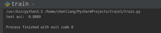
total_correct = 0
for x,y in test_loader:
    x = x.view(x.size(0), 28*28)
    out = net(x)
    #out: [b, 10] = > pred: 就会返回[b]
    pred   =out.argmax(dim=1)#返回 out 维度值最大的索引 ，也就是10那个维度
    '''
    correct 当前预测对的总个数
    pred.eq(y) :会进行比较，返回一个掩码，哪些是对等的，哪些不是。
    pred.eq(y).sum() #对等的，即1的总个数
    '''
    correct = pred.eq(y).sum().float().item()
    total_correct += correct

total_num = len(test_loader.dataset)
acc = total_correct / total_num
print('test acc: ', acc)

 

 

 

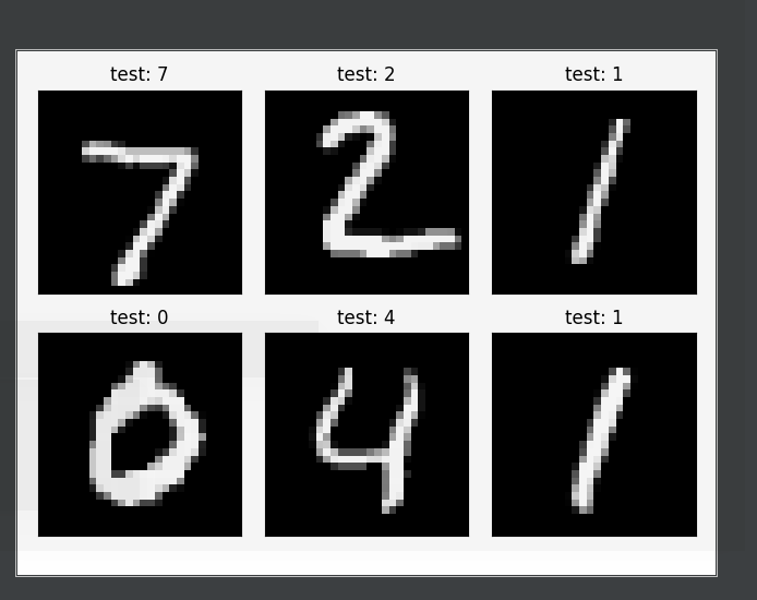
x,y  = next(iter(test_loader))
out = net(x.view(x.size(0), 28*28))
pred = out.argmax(dim=1)
plot_image(x, pred, 'test')#x:为图像 pred 为预测的数值 ,test 为名称