

Python时间序列分析
时间序列与时间序列分析
在生产和科学研究中,对某一个或者一组变量 进行观察测量,将在一系列时刻所得到的离散数字组成的序列集合,称之为时间序列。
时间序列分析是根据系统观察得到的时间序列数据,通过曲线拟合和参数估计来建立数学模型的理论和方法。时间序列分析常用于国民宏观经济控制、市场潜力预测、气象预测、农作物害虫灾害预报等各个方面。
Pandas生成时间序列:
import pandas as pd
import numpy as np
时间序列
- 时间戳(timestamp)
- 固定周期(period)
- 时间间隔(interval)
date_range
- 可以指定开始时间与周期
- H:小时
- D:天
- M:月
# TIMES的几种书写方式 #2016 Jul 1; 7/1/2016; 1/7/2016 ;2016-07-01; 2016/07/01
rng = pd.date_range('2016-07-01', periods = 10, freq = '3D')#不传freq则默认是D
rng
结果:


DatetimeIndex(['2016-07-01', '2016-07-04', '2016-07-07', '2016-07-10',
               '2016-07-13', '2016-07-16', '2016-07-19', '2016-07-22',
               '2016-07-25', '2016-07-28'],
              dtype='datetime64[ns]', freq='3D')
time=pd.Series(np.random.randn(20),
           index=pd.date_range(dt.datetime(2016,1,1),periods=20))
print(time)
#结果:
2016-01-01   -0.129379
2016-01-02    0.164480
2016-01-03   -0.639117
2016-01-04   -0.427224
2016-01-05    2.055133
2016-01-06    1.116075
2016-01-07    0.357426
2016-01-08    0.274249
2016-01-09    0.834405
2016-01-10   -0.005444
2016-01-11   -0.134409
2016-01-12    0.249318
2016-01-13   -0.297842
2016-01-14   -0.128514
2016-01-15    0.063690
2016-01-16   -2.246031
2016-01-17    0.359552
2016-01-18    0.383030
2016-01-19    0.402717
2016-01-20   -0.694068
Freq: D, dtype: float64
truncate过滤
time.truncate(before='2016-1-10')#1月10之前的都被过滤掉了
结果:
2016-01-10   -0.005444
2016-01-11   -0.134409
2016-01-12    0.249318
2016-01-13   -0.297842
2016-01-14   -0.128514
2016-01-15    0.063690
2016-01-16   -2.246031
2016-01-17    0.359552
2016-01-18    0.383030
2016-01-19    0.402717
2016-01-20   -0.694068
Freq: D, dtype: float64
time.truncate(after='2016-1-10')#1月10之后的都被过滤掉了
#结果:
2016-01-01   -0.129379
2016-01-02    0.164480
2016-01-03   -0.639117
2016-01-04   -0.427224
2016-01-05    2.055133
2016-01-06    1.116075
2016-01-07    0.357426
2016-01-08    0.274249
2016-01-09    0.834405
2016-01-10   -0.005444
Freq: D, dtype: float64
print(time['2016-01-15'])#0.063690487247
print(time['2016-01-15':'2016-01-20'])
结果:
2016-01-15    0.063690
2016-01-16   -2.246031
2016-01-17    0.359552
2016-01-18    0.383030
2016-01-19    0.402717
2016-01-20   -0.694068
Freq: D, dtype: float64


data=pd.date_range('2010-01-01','2011-01-01',freq='M')
print(data)
#结果:
DatetimeIndex(['2010-01-31', '2010-02-28', '2010-03-31', '2010-04-30',
               '2010-05-31', '2010-06-30', '2010-07-31', '2010-08-31',
               '2010-09-30', '2010-10-31', '2010-11-30', '2010-12-31'],
              dtype='datetime64[ns]', freq='M')
#时间戳
pd.Timestamp('2016-07-10')#Timestamp('2016-07-10 00:00:00')
# 可以指定更多细节
pd.Timestamp('2016-07-10 10')#Timestamp('2016-07-10 10:00:00')
pd.Timestamp('2016-07-10 10:15')#Timestamp('2016-07-10 10:15:00')

# How much detail can you add?
t = pd.Timestamp('2016-07-10 10:15')

# 时间区间
pd.Period('2016-01')#Period('2016-01', 'M')
pd.Period('2016-01-01')#Period('2016-01-01', 'D')

# TIME OFFSETS
pd.Timedelta('1 day')#Timedelta('1 days 00:00:00')
pd.Period('2016-01-01 10:10') + pd.Timedelta('1 day')#Period('2016-01-02 10:10', 'T')
pd.Timestamp('2016-01-01 10:10') + pd.Timedelta('1 day')#Timestamp('2016-01-02 10:10:00')
pd.Timestamp('2016-01-01 10:10') + pd.Timedelta('15 ns')#Timestamp('2016-01-01 10:10:00.000000015')

p1 = pd.period_range('2016-01-01 10:10', freq = '25H', periods = 10)
p2 = pd.period_range('2016-01-01 10:10', freq = '1D1H', periods = 10)
p1
p2
结果:
PeriodIndex(['2016-01-01 10:00', '2016-01-02 11:00', '2016-01-03 12:00',
             '2016-01-04 13:00', '2016-01-05 14:00', '2016-01-06 15:00',
             '2016-01-07 16:00', '2016-01-08 17:00', '2016-01-09 18:00',
             '2016-01-10 19:00'],
            dtype='period[25H]', freq='25H')
PeriodIndex(['2016-01-01 10:00', '2016-01-02 11:00', '2016-01-03 12:00',
             '2016-01-04 13:00', '2016-01-05 14:00', '2016-01-06 15:00',
             '2016-01-07 16:00', '2016-01-08 17:00', '2016-01-09 18:00',
             '2016-01-10 19:00'],
            dtype='period[25H]', freq='25H')

# 指定索引
rng = pd.date_range('2016 Jul 1', periods = 10, freq = 'D')
rng
pd.Series(range(len(rng)), index = rng)
结果:
2016-07-01    0
2016-07-02    1
2016-07-03    2
2016-07-04    3
2016-07-05    4
2016-07-06    5
2016-07-07    6
2016-07-08    7
2016-07-09    8
2016-07-10    9
Freq: D, dtype: int32

periods = [pd.Period('2016-01'), pd.Period('2016-02'), pd.Period('2016-03')]
ts = pd.Series(np.random.randn(len(periods)), index = periods)
ts
结果:
2016-01   -0.015837
2016-02   -0.923463
2016-03   -0.485212
Freq: M, dtype: float64

type(ts.index)#pandas.core.indexes.period.PeriodIndex

# 时间戳和时间周期可以转换
ts = pd.Series(range(10), pd.date_range('07-10-16 8:00', periods = 10, freq = 'H'))
ts
结果:
2016-07-10 08:00:00    0
2016-07-10 09:00:00    1
2016-07-10 10:00:00    2
2016-07-10 11:00:00    3
2016-07-10 12:00:00    4
2016-07-10 13:00:00    5
2016-07-10 14:00:00    6
2016-07-10 15:00:00    7
2016-07-10 16:00:00    8
2016-07-10 17:00:00    9
Freq: H, dtype: int32

ts_period = ts.to_period()
ts_period
结果:
2016-07-10 08:00    0
2016-07-10 09:00    1
2016-07-10 10:00    2
2016-07-10 11:00    3
2016-07-10 12:00    4
2016-07-10 13:00    5
2016-07-10 14:00    6
2016-07-10 15:00    7
2016-07-10 16:00    8
2016-07-10 17:00    9
Freq: H, dtype: int32

时间周期与时间戳的区别

ts_period['2016-07-10 08:30':'2016-07-10 11:45'] #时间周期包含08:00
结果:
2016-07-10 08:00    0
2016-07-10 09:00    1
2016-07-10 10:00    2
2016-07-10 11:00    3
Freq: H, dtype: int32

ts['2016-07-10 08:30':'2016-07-10 11:45'] #时间戳不包含08:30
#结果:
2016-07-10 09:00:00    1
2016-07-10 10:00:00    2
2016-07-10 11:00:00    3
Freq: H, dtype: int32
数据重采样:
- 时间数据由一个频率转换到另一个频率
- 降采样
- 升采样
import pandas as pd
import numpy as np
rng = pd.date_range('1/1/2011', periods=90, freq='D')#数据按天
ts = pd.Series(np.random.randn(len(rng)), index=rng)
ts.head()
结果:
2011-01-01   -1.025562
2011-01-02    0.410895
2011-01-03    0.660311
2011-01-04    0.710293
2011-01-05    0.444985
Freq: D, dtype: float64

ts.resample('M').sum()#数据降采样,降为月,指标是求和,也可以平均,自己指定
结果:
2011-01-31    2.510102
2011-02-28    0.583209
2011-03-31    2.749411
Freq: M, dtype: float64

ts.resample('3D').sum()#数据降采样,降为3天
结果:
2011-01-01    0.045643
2011-01-04   -2.255206
2011-01-07    0.571142
2011-01-10    0.835032
2011-01-13   -0.396766
2011-01-16   -1.156253
2011-01-19   -1.286884
2011-01-22    2.883952
2011-01-25    1.566908
2011-01-28    1.435563
2011-01-31    0.311565
2011-02-03   -2.541235
2011-02-06    0.317075
2011-02-09    1.598877
2011-02-12   -1.950509
2011-02-15    2.928312
2011-02-18   -0.733715
2011-02-21    1.674817
2011-02-24   -2.078872
2011-02-27    2.172320
2011-03-02   -2.022104
2011-03-05   -0.070356
2011-03-08    1.276671
2011-03-11   -2.835132
2011-03-14   -1.384113
2011-03-17    1.517565
2011-03-20   -0.550406
2011-03-23    0.773430
2011-03-26    2.244319
2011-03-29    2.951082
Freq: 3D, dtype: float64

day3Ts = ts.resample('3D').mean()
day3Ts
结果:
2011-01-01    0.015214
2011-01-04   -0.751735
2011-01-07    0.190381
2011-01-10    0.278344
2011-01-13   -0.132255
2011-01-16   -0.385418
2011-01-19   -0.428961
2011-01-22    0.961317
2011-01-25    0.522303
2011-01-28    0.478521
2011-01-31    0.103855
2011-02-03   -0.847078
2011-02-06    0.105692
2011-02-09    0.532959
2011-02-12   -0.650170
2011-02-15    0.976104
2011-02-18   -0.244572
2011-02-21    0.558272
2011-02-24   -0.692957
2011-02-27    0.724107
2011-03-02   -0.674035
2011-03-05   -0.023452
2011-03-08    0.425557
2011-03-11   -0.945044
2011-03-14   -0.461371
2011-03-17    0.505855
2011-03-20   -0.183469
2011-03-23    0.257810
2011-03-26    0.748106
2011-03-29    0.983694
Freq: 3D, dtype: float64

print(day3Ts.resample('D').asfreq())#升采样,要进行插值
结果:
2011-01-01    0.015214
2011-01-02         NaN
2011-01-03         NaN
2011-01-04   -0.751735
2011-01-05         NaN
2011-01-06         NaN
2011-01-07    0.190381
2011-01-08         NaN
2011-01-09         NaN
2011-01-10    0.278344
2011-01-11         NaN
2011-01-12         NaN
2011-01-13   -0.132255
2011-01-14         NaN
2011-01-15         NaN
2011-01-16   -0.385418
2011-01-17         NaN
2011-01-18         NaN
2011-01-19   -0.428961
2011-01-20         NaN
2011-01-21         NaN
2011-01-22    0.961317
2011-01-23         NaN
2011-01-24         NaN
2011-01-25    0.522303
2011-01-26         NaN
2011-01-27         NaN
2011-01-28    0.478521
2011-01-29         NaN
2011-01-30         NaN
                ...
2011-02-28         NaN
2011-03-01         NaN
2011-03-02   -0.674035
2011-03-03         NaN
2011-03-04         NaN
2011-03-05   -0.023452
2011-03-06         NaN
2011-03-07         NaN
2011-03-08    0.425557
2011-03-09         NaN
2011-03-10         NaN
2011-03-11   -0.945044
2011-03-12         NaN
2011-03-13         NaN
2011-03-14   -0.461371
2011-03-15         NaN
2011-03-16         NaN
2011-03-17    0.505855
2011-03-18         NaN
2011-03-19         NaN
2011-03-20   -0.183469
2011-03-21         NaN
2011-03-22         NaN
2011-03-23    0.257810
2011-03-24         NaN
2011-03-25         NaN
2011-03-26    0.748106
2011-03-27         NaN
2011-03-28         NaN
2011-03-29    0.983694
Freq: D, Length: 88, dtype: float64
插值方法:
- ffill 空值取前面的值
- bfill 空值取后面的值
- interpolate 线性取值
day3Ts.resample('D').ffill(1)
结果:
2011-01-01    0.015214
2011-01-02    0.015214
2011-01-03         NaN
2011-01-04   -0.751735
2011-01-05   -0.751735
2011-01-06         NaN
2011-01-07    0.190381
2011-01-08    0.190381
2011-01-09         NaN
2011-01-10    0.278344
2011-01-11    0.278344
2011-01-12         NaN
2011-01-13   -0.132255
2011-01-14   -0.132255
2011-01-15         NaN
2011-01-16   -0.385418
2011-01-17   -0.385418
2011-01-18         NaN
2011-01-19   -0.428961
2011-01-20   -0.428961
2011-01-21         NaN
2011-01-22    0.961317
2011-01-23    0.961317
2011-01-24         NaN
2011-01-25    0.522303
2011-01-26    0.522303
2011-01-27         NaN
2011-01-28    0.478521
2011-01-29    0.478521
2011-01-30         NaN
                ...
2011-02-28    0.724107
2011-03-01         NaN
2011-03-02   -0.674035
2011-03-03   -0.674035
2011-03-04         NaN
2011-03-05   -0.023452
2011-03-06   -0.023452
2011-03-07         NaN
2011-03-08    0.425557
2011-03-09    0.425557
2011-03-10         NaN
2011-03-11   -0.945044
2011-03-12   -0.945044
2011-03-13         NaN
2011-03-14   -0.461371
2011-03-15   -0.461371
2011-03-16         NaN
2011-03-17    0.505855
2011-03-18    0.505855
2011-03-19         NaN
2011-03-20   -0.183469
2011-03-21   -0.183469
2011-03-22         NaN
2011-03-23    0.257810
2011-03-24    0.257810
2011-03-25         NaN
2011-03-26    0.748106
2011-03-27    0.748106
2011-03-28         NaN
2011-03-29    0.983694
Freq: D, Length: 88, dtype: float64

day3Ts.resample('D').bfill(1)
结果:
2011-01-01    0.015214
2011-01-02         NaN
2011-01-03   -0.751735
2011-01-04   -0.751735
2011-01-05         NaN
2011-01-06    0.190381
2011-01-07    0.190381
2011-01-08         NaN
2011-01-09    0.278344
2011-01-10    0.278344
2011-01-11         NaN
2011-01-12   -0.132255
2011-01-13   -0.132255
2011-01-14         NaN
2011-01-15   -0.385418
2011-01-16   -0.385418
2011-01-17         NaN
2011-01-18   -0.428961
2011-01-19   -0.428961
2011-01-20         NaN
2011-01-21    0.961317
2011-01-22    0.961317
2011-01-23         NaN
2011-01-24    0.522303
2011-01-25    0.522303
2011-01-26         NaN
2011-01-27    0.478521
2011-01-28    0.478521
2011-01-29         NaN
2011-01-30    0.103855
                ...
2011-02-28         NaN
2011-03-01   -0.674035
2011-03-02   -0.674035
2011-03-03         NaN
2011-03-04   -0.023452
2011-03-05   -0.023452
2011-03-06         NaN
2011-03-07    0.425557
2011-03-08    0.425557
2011-03-09         NaN
2011-03-10   -0.945044
2011-03-11   -0.945044
2011-03-12         NaN
2011-03-13   -0.461371
2011-03-14   -0.461371
2011-03-15         NaN
2011-03-16    0.505855
2011-03-17    0.505855
2011-03-18         NaN
2011-03-19   -0.183469
2011-03-20   -0.183469
2011-03-21         NaN
2011-03-22    0.257810
2011-03-23    0.257810
2011-03-24         NaN
2011-03-25    0.748106
2011-03-26    0.748106
2011-03-27         NaN
2011-03-28    0.983694
2011-03-29    0.983694
Freq: D, Length: 88, dtype: float64

day3Ts.resample('D').interpolate('linear')#线性拟合填充
结果:
2011-01-01    0.015214
2011-01-02   -0.240435
2011-01-03   -0.496085
2011-01-04   -0.751735
2011-01-05   -0.437697
2011-01-06   -0.123658
2011-01-07    0.190381
2011-01-08    0.219702
2011-01-09    0.249023
2011-01-10    0.278344
2011-01-11    0.141478
2011-01-12    0.004611
2011-01-13   -0.132255
2011-01-14   -0.216643
2011-01-15   -0.301030
2011-01-16   -0.385418
2011-01-17   -0.399932
2011-01-18   -0.414447
2011-01-19   -0.428961
2011-01-20    0.034465
2011-01-21    0.497891
2011-01-22    0.961317
2011-01-23    0.814979
2011-01-24    0.668641
2011-01-25    0.522303
2011-01-26    0.507709
2011-01-27    0.493115
2011-01-28    0.478521
2011-01-29    0.353632
2011-01-30    0.228744
                ...
2011-02-28    0.258060
2011-03-01   -0.207988
2011-03-02   -0.674035
2011-03-03   -0.457174
2011-03-04   -0.240313
2011-03-05   -0.023452
2011-03-06    0.126218
2011-03-07    0.275887
2011-03-08    0.425557
2011-03-09   -0.031310
2011-03-10   -0.488177
2011-03-11   -0.945044
2011-03-12   -0.783820
2011-03-13   -0.622595
2011-03-14   -0.461371
2011-03-15   -0.138962
2011-03-16    0.183446
2011-03-17    0.505855
2011-03-18    0.276080
2011-03-19    0.046306
2011-03-20   -0.183469
2011-03-21   -0.036376
2011-03-22    0.110717
2011-03-23    0.257810
2011-03-24    0.421242
2011-03-25    0.584674
2011-03-26    0.748106
2011-03-27    0.826636
2011-03-28    0.905165
2011-03-29    0.983694
Freq: D, Length: 88, dtype: float64
Pandas滑动窗口:
滑动窗口就是能够根据指定的单位长度来框住时间序列,从而计算框内的统计指标。相当于一个长度指定的滑块在刻度尺上面滑动,每滑动一个单位即可反馈滑块内的数据。
滑动窗口可以使数据更加平稳,浮动范围会比较小,具有代表性,单独拿出一个数据可能或多或少会离群,有差异或者错误,使用滑动窗口会更规范一些。
%matplotlib inline
import matplotlib.pylab
import numpy as np
import pandas as pd
df = pd.Series(np.random.randn(600), index = pd.date_range('7/1/2016', freq = 'D', periods = 600))
df.head()
结果:
2016-07-01   -0.192140
2016-07-02    0.357953
2016-07-03   -0.201847
2016-07-04   -0.372230
2016-07-05    1.414753
Freq: D, dtype: float64

r = df.rolling(window = 10)
r#Rolling [window=10,center=False,axis=0]

#r.max, r.median, r.std, r.skew倾斜度, r.sum, r.var
print(r.mean())
结果:
2016-07-01         NaN
2016-07-02         NaN
2016-07-03         NaN
2016-07-04         NaN
2016-07-05         NaN
2016-07-06         NaN
2016-07-07         NaN
2016-07-08         NaN
2016-07-09         NaN
2016-07-10    0.300133
2016-07-11    0.284780
2016-07-12    0.252831
2016-07-13    0.220699
2016-07-14    0.167137
2016-07-15    0.018593
2016-07-16   -0.061414
2016-07-17   -0.134593
2016-07-18   -0.153333
2016-07-19   -0.218928
2016-07-20   -0.169426
2016-07-21   -0.219747
2016-07-22   -0.181266
2016-07-23   -0.173674
2016-07-24   -0.130629
2016-07-25   -0.166730
2016-07-26   -0.233044
2016-07-27   -0.256642
2016-07-28   -0.280738
2016-07-29   -0.289893
2016-07-30   -0.379625
                ...
2018-01-22   -0.211467
2018-01-23    0.034996
2018-01-24   -0.105910
2018-01-25   -0.145774
2018-01-26   -0.089320
2018-01-27   -0.164370
2018-01-28   -0.110892
2018-01-29   -0.205786
2018-01-30   -0.101162
2018-01-31   -0.034760
2018-02-01    0.229333
2018-02-02    0.043741
2018-02-03    0.052837
2018-02-04    0.057746
2018-02-05   -0.071401
2018-02-06   -0.011153
2018-02-07   -0.045737
2018-02-08   -0.021983
2018-02-09   -0.196715
2018-02-10   -0.063721
2018-02-11   -0.289452
2018-02-12   -0.050946
2018-02-13   -0.047014
2018-02-14    0.048754
2018-02-15    0.143949
2018-02-16    0.424823
2018-02-17    0.361878
2018-02-18    0.363235
2018-02-19    0.517436
2018-02-20    0.368020
Freq: D, Length: 600, dtype: float64

import matplotlib.pyplot as plt
%matplotlib inline

plt.figure(figsize=(15, 5))

df.plot(style='r--')
df.rolling(window=10).mean().plot(style='b')#<matplotlib.axes._subplots.AxesSubplot at 0x249627fb6d8>
结果:

数据平稳性与差分法:
基本模型:自回归移动平均模型(ARMA(p,q))是时间序列中最为重要的模型之一。它主要由两部分组成: AR代表p阶自回归过程,MA代表q阶移动平均过程。

平稳性检验
我们知道序列平稳性是进行时间序列分析的前提条件,很多人都会有疑问,为什么要满足平稳性的要求呢?在大数定理和中心定理中要求样本同分布(这里同分布等价于时间序列中的平稳性),而我们的建模过程中有很多都是建立在大数定理和中心极限定理的前提条件下的,如果它不满足,得到的许多结论都是不可靠的。以虚假回归为例,当响应变量和输入变量都平稳时,我们用t统计量检验标准化系数的显著性。而当响应变量和输入变量不平稳时,其标准化系数不在满足t分布,这时再用t检验来进行显著性分析,导致拒绝原假设的概率增加,即容易犯第一类错误,从而得出错误的结论。
平稳时间序列有两种定义:严平稳和宽平稳

严平稳顾名思义,是一种条件非常苛刻的平稳性,它要求序列随着时间的推移,其统计性质保持不变。对于任意的τ,其联合概率密度函数满足:

严平稳的条件只是理论上的存在,现实中用得比较多的是宽平稳的条件。
宽平稳也叫弱平稳或者二阶平稳(均值和方差平稳),它应满足:
- 常数均值
- 常数方差
- 常数自协方差
ARIMA 模型对时间序列的要求是平稳型。因此,当你得到一个非平稳的时间序列时,首先要做的即是做时间序列的差分,直到得到一个平稳时间序列。如果你对时间序列做d次差分才能得到一个平稳序列,那么可以使用ARIMA(p,d,q)模型,其中d是差分次数。

二阶差分是指在一阶差分基础上再做一阶差分。
%load_ext autoreload
%autoreload 2
%matplotlib inline
%config InlineBackend.figure_format='retina'

from __future__ import absolute_import, division, print_function
# http://www.lfd.uci.edu/~gohlke/pythonlibs/#xgboost各种python库文件的下载,基本可以找到所有的
import sys
import os

import pandas as pd
import numpy as np

# # Remote Data Access
# import pandas_datareader.data as web
# import datetime
# # reference: https://pandas-datareader.readthedocs.io/en/latest/remote_data.html

# TSA from Statsmodels
import statsmodels.api as sm
import statsmodels.formula.api as smf
import statsmodels.tsa.api as smt

# Display and Plotting
import matplotlib.pylab as plt
import seaborn as sns

pd.set_option('display.float_format', lambda x: '%.5f' % x) # pandas
np.set_printoptions(precision=5, suppress=True) # numpy

pd.set_option('display.max_columns', 100)
pd.set_option('display.max_rows', 100)

# seaborn plotting style
sns.set(style='ticks', context='poster')
结果:
The autoreload extension is already loaded. To reload it, use:
  %reload_ext autoreload
#Read the data
#美国消费者信心指数
Sentiment = 'data/sentiment.csv'
Sentiment = pd.read_csv(Sentiment, index_col=0, parse_dates=[0])
Sentiment.head()
结果:
| UMCSENT | |
|---|---|
| DATE | |
| 2000-01-01 | 112.00000 |
| 2000-02-01 | 111.30000 |
| 2000-03-01 | 107.10000 |
| 2000-04-01 | 109.20000 |
| 2000-05-01 | 110.70000 |
# Select the series from 2005 - 2016
sentiment_short = Sentiment.loc['2005':'2016']
sentiment_short.plot(figsize=(12,8))
plt.legend(bbox_to_anchor=(1.25, 0.5))
plt.title("Consumer Sentiment")
sns.despine()
结果:

sentiment_short['diff_1'] = sentiment_short['UMCSENT'].diff(1)#求差分值,一阶差分。     1指的是1个时间间隔,可更改。

sentiment_short['diff_2'] = sentiment_short['diff_1'].diff(1)#再求差分,二阶差分。

sentiment_short.plot(subplots=True, figsize=(18, 12))
结果:
array([<matplotlib.axes._subplots.AxesSubplot object at 0x000001D9383BACF8>,
       <matplotlib.axes._subplots.AxesSubplot object at 0x000001D939FAB6A0>,
       <matplotlib.axes._subplots.AxesSubplot object at 0x000001D93A139B70>], dtype=object)

ARIMA模型:


相关函数评估方法:
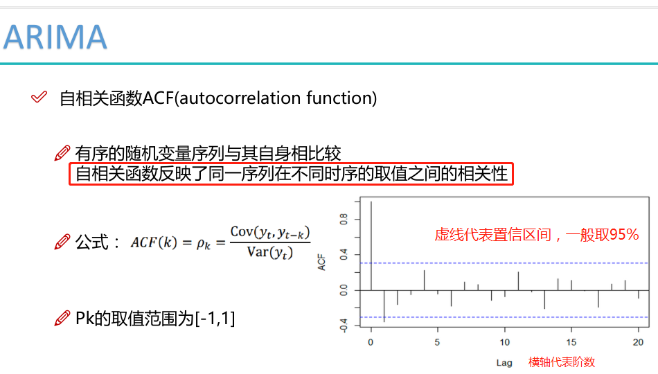

通过ACF和PACF的图选择出p值和q值。
建立ARIMA模型:
del sentiment_short['diff_2']
del sentiment_short['diff_1']
sentiment_short.head()
print (type(sentiment_short))#<class 'pandas.core.frame.DataFrame'>
fig = plt.figure(figsize=(12,8))
#acf
ax1 = fig.add_subplot(211)
fig = sm.graphics.tsa.plot_acf(sentiment_short, lags=20,ax=ax1)
ax1.xaxis.set_ticks_position('bottom')
fig.tight_layout();
#pacf
ax2 = fig.add_subplot(212)
fig = sm.graphics.tsa.plot_pacf(sentiment_short, lags=20, ax=ax2)
ax2.xaxis.set_ticks_position('bottom')
fig.tight_layout();
#下图中的阴影表示置信区间,可以看出不同阶数自相关性的变化情况,从而选出p值和q值
结果:


# 散点图也可以表示

lags=9

ncols=3
nrows=int(np.ceil(lags/ncols))

fig, axes = plt.subplots(ncols=ncols, nrows=nrows, figsize=(4*ncols, 4*nrows))

for ax, lag in zip(axes.flat, np.arange(1,lags+1, 1)):
    lag_str = 't-{}'.format(lag)
    X = (pd.concat([sentiment_short, sentiment_short.shift(-lag)], axis=1,
                   keys=['y'] + [lag_str]).dropna())

    X.plot(ax=ax, kind='scatter', y='y', x=lag_str);
    corr = X.corr().as_matrix()[0][1]
    ax.set_ylabel('Original')
    ax.set_title('Lag: {} (corr={:.2f})'.format(lag_str, corr));
    ax.set_aspect('equal');
    sns.despine();

fig.tight_layout();
结果:

# 更直观一些
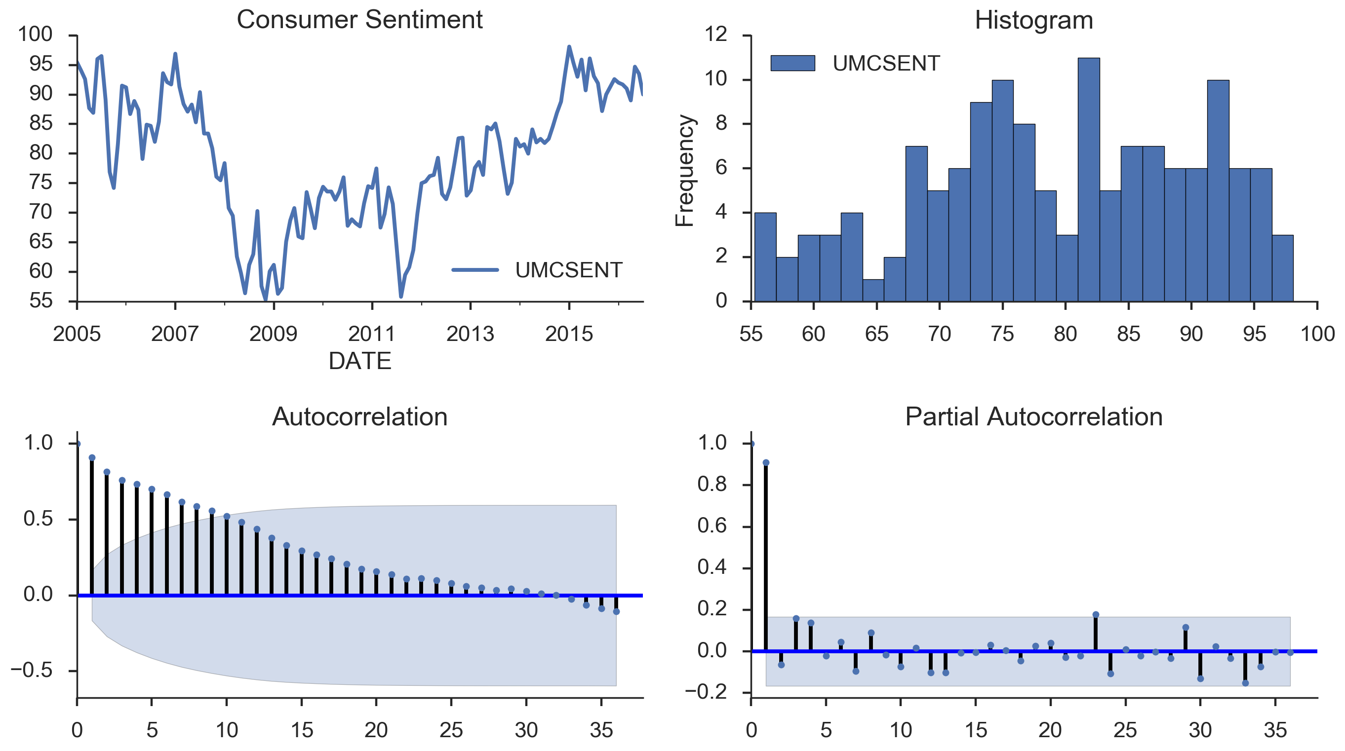
#模板,使用时直接改自己的数据就行,用以下四个图进行评估和分析就可以
def tsplot(y, lags=None, title='', figsize=(14, 8)):
fig = plt.figure(figsize=figsize)
layout = (2, 2)
ts_ax = plt.subplot2grid(layout, (0, 0))
hist_ax = plt.subplot2grid(layout, (0, 1))
acf_ax = plt.subplot2grid(layout, (1, 0))
pacf_ax = plt.subplot2grid(layout, (1, 1))
y.plot(ax=ts_ax)
ts_ax.set_title(title)
y.plot(ax=hist_ax, kind='hist', bins=25)
hist_ax.set_title('Histogram')
smt.graphics.plot_acf(y, lags=lags, ax=acf_ax)
smt.graphics.plot_pacf(y, lags=lags, ax=pacf_ax)
[ax.set_xlim(0) for ax in [acf_ax, pacf_ax]]
sns.despine()
plt.tight_layout()
return ts_ax, acf_ax, pacf_ax
tsplot(sentiment_short, title='Consumer Sentiment', lags=36);
结果:
参数选择:


BIC的结果受样本的影响,使用同一样本时,可以选择BIC。
%load_ext autoreload
%autoreload 2
%matplotlib inline
%config InlineBackend.figure_format='retina'

from __future__ import absolute_import, division, print_function

import sys
import os

import pandas as pd
import numpy as np

# TSA from Statsmodels
import statsmodels.api as sm
import statsmodels.formula.api as smf
import statsmodels.tsa.api as smt

# Display and Plotting
import matplotlib.pylab as plt
import seaborn as sns

pd.set_option('display.float_format', lambda x: '%.5f' % x) # pandas
np.set_printoptions(precision=5, suppress=True) # numpy

pd.set_option('display.max_columns', 100)
pd.set_option('display.max_rows', 100)

# seaborn plotting style
sns.set(style='ticks', context='poster')
filename_ts = 'data/series1.csv'
ts_df = pd.read_csv(filename_ts, index_col=0, parse_dates=[0])

n_sample = ts_df.shape[0]
print(ts_df.shape)
print(ts_df.head())
结果:
(120, 1)
              value
2006-06-01  0.21507
2006-07-01  1.14225
2006-08-01  0.08077
2006-09-01 -0.73952
2006-10-01  0.53552
# Create a training sample and testing sample before analyzing the series

n_train=int(0.95*n_sample)+1
n_forecast=n_sample-n_train
#ts_df
ts_train = ts_df.iloc[:n_train]['value']
ts_test = ts_df.iloc[n_train:]['value']
print(ts_train.shape)
print(ts_test.shape)
print("Training Series:", "\n", ts_train.tail(), "\n")
print("Testing Series:", "\n", ts_test.head())
结果:
(115,)
(5,)
Training Series:
 2015-08-01    0.60371
2015-09-01   -1.27372
2015-10-01   -0.93284
2015-11-01    0.08552
2015-12-01    1.20534
Name: value, dtype: float64

Testing Series:
 2016-01-01    2.16411
2016-02-01    0.95226
2016-03-01    0.36485
2016-04-01   -2.26487
2016-05-01   -2.38168
Name: value, dtype: float64
def tsplot(y, lags=None, title='', figsize=(14, 8)):

    fig = plt.figure(figsize=figsize)
    layout = (2, 2)
    ts_ax   = plt.subplot2grid(layout, (0, 0))
    hist_ax = plt.subplot2grid(layout, (0, 1))
    acf_ax  = plt.subplot2grid(layout, (1, 0))
    pacf_ax = plt.subplot2grid(layout, (1, 1))

    y.plot(ax=ts_ax)
    ts_ax.set_title(title)
    y.plot(ax=hist_ax, kind='hist', bins=25)
    hist_ax.set_title('Histogram')
    smt.graphics.plot_acf(y, lags=lags, ax=acf_ax)
    smt.graphics.plot_pacf(y, lags=lags, ax=pacf_ax)
    [ax.set_xlim(0) for ax in [acf_ax, pacf_ax]]
    sns.despine()
    fig.tight_layout()
    return ts_ax, acf_ax, pacf_ax
tsplot(ts_train, title='A Given Training Series', lags=20);
结果:

#Model Estimation

# Fit the model
arima200 = sm.tsa.SARIMAX(ts_train, order=(2,0,0))#order里边的三个参数p,d,q
model_results = arima200.fit()#fit模型
import itertools
#当多组值都不符合时,遍历多组值,得出最好的值
p_min = 0
d_min = 0
q_min = 0
p_max = 4
d_max = 0
q_max = 4

# Initialize a DataFrame to store the results
results_bic = pd.DataFrame(index=['AR{}'.format(i) for i in range(p_min,p_max+1)],
                           columns=['MA{}'.format(i) for i in range(q_min,q_max+1)])

for p,d,q in itertools.product(range(p_min,p_max+1),
                               range(d_min,d_max+1),
                               range(q_min,q_max+1)):
    if p==0 and d==0 and q==0:
        results_bic.loc['AR{}'.format(p), 'MA{}'.format(q)] = np.nan
        continue

    try:
        model = sm.tsa.SARIMAX(ts_train, order=(p, d, q),
                               #enforce_stationarity=False,
                               #enforce_invertibility=False,
                              )
        results = model.fit()
        results_bic.loc['AR{}'.format(p), 'MA{}'.format(q)] = results.bic
    except:
        continue
results_bic = results_bic[results_bic.columns].astype(float)
fig, ax = plt.subplots(figsize=(10, 8))
ax = sns.heatmap(results_bic,
                 mask=results_bic.isnull(),
                 ax=ax,
                 annot=True,
                 fmt='.2f',
                 );
ax.set_title('BIC');
结果:

# Alternative model selection method, limited to only searching AR and MA parameters

train_results = sm.tsa.arma_order_select_ic(ts_train, ic=['aic', 'bic'], trend='nc', max_ar=4, max_ma=4)

print('AIC', train_results.aic_min_order)
print('BIC', train_results.bic_min_order)
结果:得出两个不同的标准,比较尴尬,还需要进行筛选
AIC (4, 2)
BIC (1, 1)

#残差分析 正态分布 QQ图线性
model_results.plot_diagnostics(figsize=(16, 12));#statsmodels库
结果:

Q-Q图:越像直线,则是正态分布;越不是直线,离正态分布越远。
时间序列建模基本步骤:
- 获取被观测系统时间序列数据;
- 对数据绘图,观测是否为平稳时间序列;对于非平稳时间序列要先进行d阶差分运算,化为平稳时间序列;
- 经过第二步处理,已经得到平稳时间序列。要对平稳时间序列分别求得其自相关系数ACF 和偏自相关系数PACF ,通过对自相关图和偏自相关图的分析,得到最佳的阶层 p 和阶数 q
- 由以上得到的 ,得到ARIMA模型。然后开始对得到的模型进行模型检验。
股票预测(属于回归):
%matplotlib inline
import pandas as pd
import pandas_datareader#用于从雅虎财经获取股票数据
import datetime
import matplotlib.pylab as plt
import seaborn as sns
from matplotlib.pylab import style
from statsmodels.tsa.arima_model import ARIMA
from statsmodels.graphics.tsaplots import plot_acf, plot_pacf

style.use('ggplot')
plt.rcParams['font.sans-serif'] = ['SimHei']
plt.rcParams['axes.unicode_minus'] = False
stockFile = 'data/T10yr.csv'
stock = pd.read_csv(stockFile, index_col=0, parse_dates=[0])#将索引index设置为时间,parse_dates对日期格式处理为标准格式。
stock.head(10)
结果:
| Open | High | Low | Close | Volume | Adj Close | |
|---|---|---|---|---|---|---|
| Date | ||||||
| 2000-01-03 | 6.498 | 6.603 | 6.498 | 6.548 | 0 | 6.548 |
| 2000-01-04 | 6.530 | 6.548 | 6.485 | 6.485 | 0 | 6.485 |
| 2000-01-05 | 6.521 | 6.599 | 6.508 | 6.599 | 0 | 6.599 |
| 2000-01-06 | 6.558 | 6.585 | 6.540 | 6.549 | 0 | 6.549 |
| 2000-01-07 | 6.545 | 6.595 | 6.504 | 6.504 | 0 | 6.504 |
| 2000-01-10 | 6.540 | 6.567 | 6.536 | 6.558 | 0 | 6.558 |
| 2000-01-11 | 6.600 | 6.664 | 6.595 | 6.664 | 0 | 6.664 |
| 2000-01-12 | 6.659 | 6.696 | 6.645 | 6.696 | 0 | 6.696 |
| 2000-01-13 | 6.664 | 6.705 | 6.618 | 6.618 | 0 | 6.618 |
| 2000-01-14 | 6.623 | 6.688 | 6.563 | 6.674 | 0 | 6.674 |
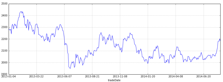
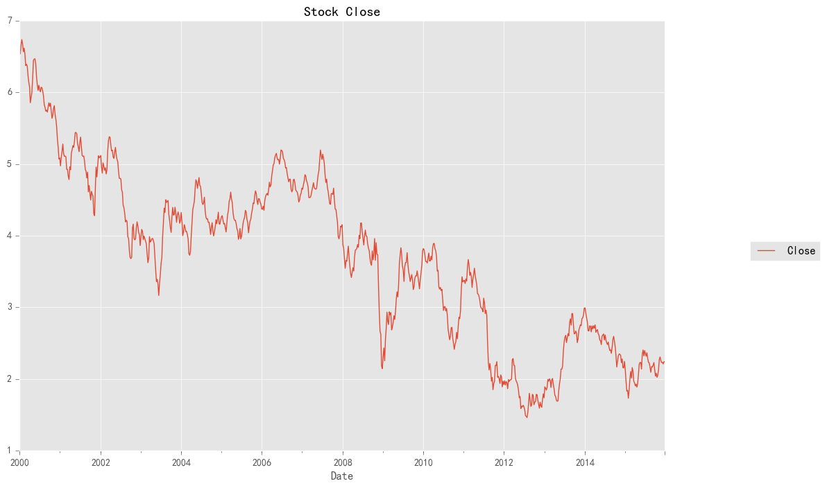
stock_week = stock['Close'].resample('W-MON').mean()
stock_train = stock_week['2000':'2015']
stock_train.plot(figsize=(12,8))
plt.legend(bbox_to_anchor=(1.25, 0.5))
plt.title("Stock Close")
sns.despine()
结果:
stock_diff = stock_train.diff()
stock_diff = stock_diff.dropna()

plt.figure()
plt.plot(stock_diff)
plt.title('一阶差分')
plt.show()
结果:

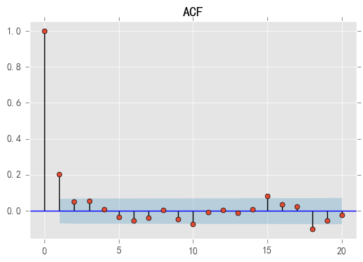
acf = plot_acf(stock_diff, lags=20)
plt.title("ACF")
acf.show()
结果:
pacf = plot_pacf(stock_diff, lags=20)
plt.title("PACF")
pacf.show()
结果:

model = ARIMA(stock_train, order=(1, 1, 1),freq='W-MON')
result = model.fit()
#print(result.summary())#统计出ARIMA模型的指标
pred = result.predict('20140609', '20160701',dynamic=True, typ='levels')#预测,指定起始与终止时间。预测值起始时间必须在原始数据中,终止时间不需要
print (pred)
结果:
2014-06-09    2.463559
2014-06-16    2.455539
2014-06-23    2.449569
2014-06-30    2.444183
2014-07-07    2.438962
2014-07-14    2.433788
2014-07-21    2.428627
2014-07-28    2.423470
2014-08-04    2.418315
2014-08-11    2.413159
2014-08-18    2.408004
2014-08-25    2.402849
2014-09-01    2.397693
2014-09-08    2.392538
2014-09-15    2.387383
2014-09-22    2.382227
2014-09-29    2.377072
2014-10-06    2.371917
2014-10-13    2.366761
2014-10-20    2.361606
2014-10-27    2.356451
2014-11-03    2.351296
2014-11-10    2.346140
2014-11-17    2.340985
2014-11-24    2.335830
2014-12-01    2.330674
2014-12-08    2.325519
2014-12-15    2.320364
2014-12-22    2.315208
2014-12-29    2.310053
                ...
2015-12-07    2.057443
2015-12-14    2.052288
2015-12-21    2.047132
2015-12-28    2.041977
2016-01-04    2.036822
2016-01-11    2.031666
2016-01-18    2.026511
2016-01-25    2.021356
2016-02-01    2.016200
2016-02-08    2.011045
2016-02-15    2.005890
2016-02-22    2.000735
2016-02-29    1.995579
2016-03-07    1.990424
2016-03-14    1.985269
2016-03-21    1.980113
2016-03-28    1.974958
2016-04-04    1.969803
2016-04-11    1.964647
2016-04-18    1.959492
2016-04-25    1.954337
2016-05-02    1.949181
2016-05-09    1.944026
2016-05-16    1.938871
2016-05-23    1.933716
2016-05-30    1.928560
2016-06-06    1.923405
2016-06-13    1.918250
2016-06-20    1.913094
2016-06-27    1.907939
Freq: W-MON, Length: 108, dtype: float64
plt.figure(figsize=(6, 6))
plt.xticks(rotation=45)
plt.plot(pred)
plt.plot(stock_train)#[<matplotlib.lines.Line2D at 0x28025665278>]
结果:

使用tfresh库进行分类任务:
tsfresh是开源的提取时序数据特征的python包,能够提取出超过64种特征,堪称提取时序特征的瑞士军刀。用到时tfresh查官方文档
%matplotlib inline
import matplotlib.pylab as plt
import seaborn as sns
from tsfresh.examples.robot_execution_failures import download_robot_execution_failures, load_robot_execution_failures
from tsfresh import extract_features, extract_relevant_features, select_features
from tsfresh.utilities.dataframe_functions import impute
from tsfresh.feature_extraction import ComprehensiveFCParameters
from sklearn.tree import DecisionTreeClassifier
from sklearn.cross_validation import train_test_split
from sklearn.metrics import classification_report


#http://tsfresh.readthedocs.io/en/latest/text/quick_start.html#官方文档
download_robot_execution_failures()
df, y = load_robot_execution_failures()
df.head()
结果:
id    time    a    b    c    d    e    f
0    1    0    -1    -1    63    -3    -1    0
1    1    1    0    0    62    -3    -1    0
2    1    2    -1    -1    61    -3    0    0
3    1    3    -1    -1    63    -2    -1    0
4    1    4    -1    -1    63    -3    -1    0
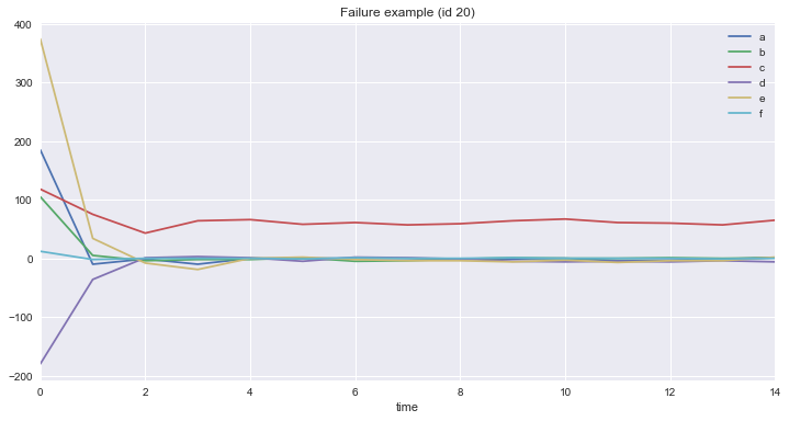
df[df.id == 3][['time', 'a', 'b', 'c', 'd', 'e', 'f']].plot(x='time', title='Success example (id 3)', figsize=(12, 6));
df[df.id == 20][['time', 'a', 'b', 'c', 'd', 'e', 'f']].plot(x='time', title='Failure example (id 20)', figsize=(12, 6));
结果:

extraction_settings = ComprehensiveFCParameters()#提取特征
#column_id (str) – The name of the id column to group by
#column_sort (str) – The name of the sort column.
X = extract_features(df,
                     column_id='id', column_sort='time',#以id为聚合,以time排序
                     default_fc_parameters=extraction_settings,
                     impute_function= impute)
X.head()#提取到的特征
结果:
a__mean_abs_change_quantiles__qh_1.0__ql_0.8    a__percentage_of_reoccurring_values_to_all_values    a__mean_abs_change_quantiles__qh_1.0__ql_0.2    a__mean_abs_change_quantiles__qh_1.0__ql_0.0    a__large_standard_deviation__r_0.45    a__absolute_sum_of_changes    a__mean_abs_change_quantiles__qh_1.0__ql_0.4    a__mean_second_derivate_central    a__autocorrelation__lag_4    a__binned_entropy__max_bins_10    ...    f__fft_coefficient__coeff_0    f__fft_coefficient__coeff_1    f__fft_coefficient__coeff_2    f__fft_coefficient__coeff_3    f__fft_coefficient__coeff_4    f__fft_coefficient__coeff_5    f__fft_coefficient__coeff_6    f__fft_coefficient__coeff_7    f__fft_coefficient__coeff_8    f__fft_coefficient__coeff_9
id
1    0.142857    0.933333    0.142857    0.142857    0.0    2.0    0.142857    -0.038462    0.17553    0.244930    ...    0.0    0.000000    0.000000    0.000000    0.000000    0.0    0.000000    0.000000    0.0    0.0
2    0.000000    1.000000    0.400000    1.000000    0.0    14.0    0.400000    -0.038462    0.17553    0.990835    ...    -4.0    0.744415    1.273659    -0.809017    1.373619    0.5    0.309017    -1.391693    0.0    0.0
3    0.000000    0.933333    0.714286    0.714286    0.0    10.0    0.714286    -0.038462    0.17553    0.729871    ...    -4.0    -0.424716    0.878188    1.000000    1.851767    0.5    1.000000    -2.805239    0.0    0.0
4    0.000000    1.000000    0.800000    1.214286    0.0    17.0    0.800000    -0.038462    0.17553    1.322950    ...    -5.0    -1.078108    3.678858    -3.618034    -1.466977    -0.5    -1.381966    -0.633773    0.0    0.0
5    2.000000    0.866667    0.916667    0.928571    0.0    13.0    0.916667    0.038462    0.17553    1.020037    ...    -2.0    -3.743460    3.049653    -0.618034    1.198375    -0.5    1.618034    -0.004568    0.0    0.0
5 rows × 1332 columns
X.info()
#结果:
<class 'pandas.core.frame.DataFrame'>
Int64Index: 88 entries, 1 to 88
Columns: 1332 entries, a__mean_abs_change_quantiles__qh_1.0__ql_0.8 to f__fft_coefficient__coeff_9
dtypes: float64(1332)
memory usage: 916.4 KB
X_filtered = extract_relevant_features(df, y,
                                       column_id='id', column_sort='time',
                                       default_fc_parameters=extraction_settings)#特征过滤,选择最相关的特征。具体了解查看官方文档
X_filtered.head()#新特征
结果:
a__abs_energy    a__range_count__max_1__min_-1    b__abs_energy    e__variance    e__standard_deviation    e__abs_energy    c__standard_deviation    c__variance    a__standard_deviation    a__variance    ...    b__has_duplicate_max    b__cwt_coefficients__widths_(2, 5, 10, 20)__coeff_14__w_5    b__cwt_coefficients__widths_(2, 5, 10, 20)__coeff_13__w_2    e__quantile__q_0.1    a__ar_coefficient__k_10__coeff_1    a__quantile__q_0.2    b__quantile__q_0.7    f__large_standard_deviation__r_0.35    f__quantile__q_0.9    d__spkt_welch_density__coeff_5
id
1    14.0    15.0    13.0    0.222222    0.471405    10.0    1.203698    1.448889    0.249444    0.062222    ...    1.0    -0.751682    -0.310265    -1.0    0.125000    -1.0    -1.0    0.0    0.0    0.037795
2    25.0    13.0    76.0    4.222222    2.054805    90.0    4.333846    18.782222    0.956847    0.915556    ...    1.0    0.057818    -0.202951    -3.6    -0.078829    -1.0    -1.0    1.0    0.0    0.319311
3    12.0    14.0    40.0    3.128889    1.768867    103.0    4.616877    21.315556    0.596285    0.355556    ...    0.0    0.912474    0.539121    -4.0    0.084836    -1.0    0.0    1.0    0.0    9.102780
4    16.0    10.0    60.0    7.128889    2.669998    124.0    3.833188    14.693333    0.952190    0.906667    ...    0.0    -0.609735    -2.641390    -4.6    0.003108    -1.0    1.0    0.0    0.0    56.910262
5    17.0    13.0    46.0    4.160000    2.039608    180.0    4.841487    23.440000    0.879394    0.773333    ...    0.0    0.072771    0.591927    -5.0    0.087906    -1.0    0.8    0.0    0.6    22.841805
5 rows × 300 columns
X_filtered.info()
结果:
<class 'pandas.core.frame.DataFrame'>
Int64Index: 88 entries, 1 to 88
Columns: 300 entries, a__abs_energy to d__spkt_welch_density__coeff_5
dtypes: float64(300)
memory usage: 206.9 KB
X_train, X_test, X_filtered_train, X_filtered_test, y_train, y_test = train_test_split(X, X_filtered, y, test_size=.4)
cl = DecisionTreeClassifier()
cl.fit(X_train, y_train)
print(classification_report(y_test, cl.predict(X_test)))#对模型进行评估,可以看出这个结果还不错
结果:
precision    recall  f1-score   support

          0       1.00      0.89      0.94         9
          1       0.96      1.00      0.98        27

avg / total       0.97      0.97      0.97        36
cl.n_features_#1332
cl2 = DecisionTreeClassifier()
cl2.fit(X_filtered_train, y_train)
print(classification_report(y_test, cl2.predict(X_filtered_test)))
结果:
cl2 = DecisionTreeClassifier()
cl2.fit(X_filtered_train, y_train)
print(classification_report(y_test, cl2.predict(X_filtered_test)))
cl2 = DecisionTreeClassifier()
cl2.fit(X_filtered_train, y_train)
print(classification_report(y_test, cl2.predict(X_filtered_test)))
             precision    recall  f1-score   support

          0       1.00      0.78      0.88         9
          1       0.93      1.00      0.96        27

avg / total       0.95      0.94      0.94        36
cl2.n_features_#300
维基百科词条EDA
探索性数据分析(EDA)目的是最大化对数据的直觉,完成这个事情的方法只能是结合统计学的图形以各种形式展现出来。通过EDA可以实现:
1. 得到数据的直观表现
2. 发现潜在的结构
3. 提取重要的变量
4. 处理异常值
5. 检验统计假设
6. 建立初步模型
7. 决定最优因子的设置
import pandas as pd
import numpy as np
import matplotlib.pyplot as plt
import re
%matplotlib inline
train = pd.read_csv('train_1.csv').fillna(0)
train.head()
结果:
Page    2015-07-01    2015-07-02    2015-07-03    2015-07-04    2015-07-05    2015-07-06    2015-07-07    2015-07-08    2015-07-09    ...    2016-12-22    2016-12-23    2016-12-24    2016-12-25    2016-12-26    2016-12-27    2016-12-28    2016-12-29    2016-12-30    2016-12-31
0    2NE1_zh.wikipedia.org_all-access_spider    18.0    11.0    5.0    13.0    14.0    9.0    9.0    22.0    26.0    ...    32.0    63.0    15.0    26.0    14.0    20.0    22.0    19.0    18.0    20.0
1    2PM_zh.wikipedia.org_all-access_spider    11.0    14.0    15.0    18.0    11.0    13.0    22.0    11.0    10.0    ...    17.0    42.0    28.0    15.0    9.0    30.0    52.0    45.0    26.0    20.0
2    3C_zh.wikipedia.org_all-access_spider    1.0    0.0    1.0    1.0    0.0    4.0    0.0    3.0    4.0    ...    3.0    1.0    1.0    7.0    4.0    4.0    6.0    3.0    4.0    17.0
3    4minute_zh.wikipedia.org_all-access_spider    35.0    13.0    10.0    94.0    4.0    26.0    14.0    9.0    11.0    ...    32.0    10.0    26.0    27.0    16.0    11.0    17.0    19.0    10.0    11.0
4    52_Hz_I_Love_You_zh.wikipedia.org_all-access_s...    0.0    0.0    0.0    0.0    0.0    0.0    0.0    0.0    0.0    ...    48.0    9.0    25.0    13.0    3.0    11.0    27.0    13.0    36.0    10.0
5 rows × 551 columns
train.info()
结果:<class 'pandas.core.frame.DataFrame'>
RangeIndex: 145063 entries, 0 to 145062
Columns: 551 entries, Page to 2016-12-31
dtypes: float64(550), object(1)
memory usage: 609.8+ MB
for col in train.columns[1:]:
    train[col] = pd.to_numeric(train[col],downcast='integer')#float数据较为占内存,从上表可以看出,小数点后都是0,可将数据转换为int,减小内存。
train.head()
结果:
Page    2015-07-01    2015-07-02    2015-07-03    2015-07-04    2015-07-05    2015-07-06    2015-07-07    2015-07-08    2015-07-09    ...    2016-12-22    2016-12-23    2016-12-24    2016-12-25    2016-12-26    2016-12-27    2016-12-28    2016-12-29    2016-12-30    2016-12-31
0    2NE1_zh.wikipedia.org_all-access_spider    18    11    5    13    14    9    9    22    26    ...    32    63    15    26    14    20    22    19    18    20
1    2PM_zh.wikipedia.org_all-access_spider    11    14    15    18    11    13    22    11    10    ...    17    42    28    15    9    30    52    45    26    20
2    3C_zh.wikipedia.org_all-access_spider    1    0    1    1    0    4    0    3    4    ...    3    1    1    7    4    4    6    3    4    17
3    4minute_zh.wikipedia.org_all-access_spider    35    13    10    94    4    26    14    9    11    ...    32    10    26    27    16    11    17    19    10    11
4    52_Hz_I_Love_You_zh.wikipedia.org_all-access_s...    0    0    0    0    0    0    0    0    0    ...    48    9    25    13    3    11    27    13    36    10
5 rows × 551 columns
train.info()
结果:
<class 'pandas.core.frame.DataFrame'>
RangeIndex: 145063 entries, 0 to 145062
Columns: 551 entries, Page to 2016-12-31
dtypes: int32(550), object(1)
memory usage: 305.5+ MB
def get_language(page):#将词条按国家分类
    res = re.search('[a-z][a-z].wikipedia.org',page)
    #print (res.group()[0:2])
    if res:
        return res.group()[0:2]
    return 'na'

train['lang'] = train.Page.map(get_language)

from collections import Counter

print(Counter(train.lang))
结果:Counter({'en': 24108, 'ja': 20431, 'de': 18547, 'na': 17855, 'fr': 17802, 'zh': 17229, 'ru': 15022, 'es': 14069})
lang_sets = {}
lang_sets['en'] = train[train.lang=='en'].iloc[:,0:-1]
lang_sets['ja'] = train[train.lang=='ja'].iloc[:,0:-1]
lang_sets['de'] = train[train.lang=='de'].iloc[:,0:-1]
lang_sets['na'] = train[train.lang=='na'].iloc[:,0:-1]
lang_sets['fr'] = train[train.lang=='fr'].iloc[:,0:-1]
lang_sets['zh'] = train[train.lang=='zh'].iloc[:,0:-1]
lang_sets['ru'] = train[train.lang=='ru'].iloc[:,0:-1]
lang_sets['es'] = train[train.lang=='es'].iloc[:,0:-1]

sums = {}
for key in lang_sets:
    sums[key] = lang_sets[key].iloc[:,1:].sum(axis=0) / lang_sets[key].shape[0]
days = [r for r in range(sums['en'].shape[0])]

fig = plt.figure(1,figsize=[10,10])
plt.ylabel('Views per Page')
plt.xlabel('Day')
plt.title('Pages in Different Languages')
labels={'en':'English','ja':'Japanese','de':'German',
        'na':'Media','fr':'French','zh':'Chinese',
        'ru':'Russian','es':'Spanish'
       }

for key in sums:
    plt.plot(days,sums[key],label = labels[key] )

plt.legend()
plt.show()
结果:

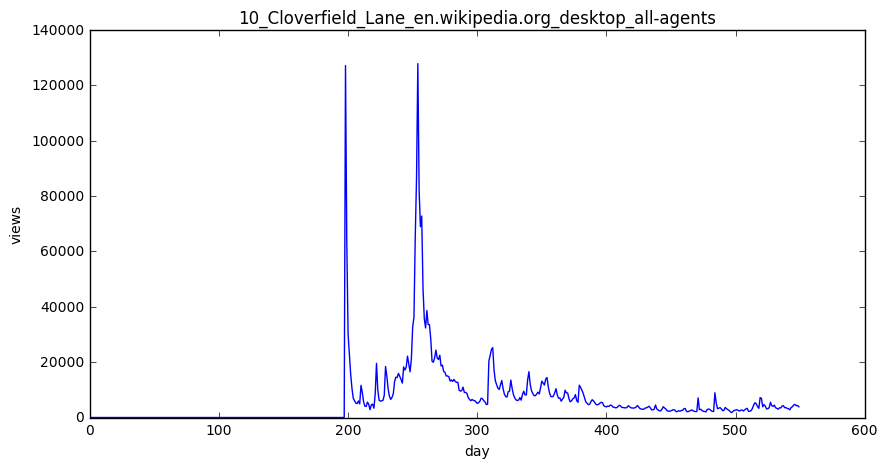
def plot_entry(key,idx):
    data = lang_sets[key].iloc[idx,1:]
    fig = plt.figure(1,figsize=(10,5))
    plt.plot(days,data)
    plt.xlabel('day')
    plt.ylabel('views')
    plt.title(train.iloc[lang_sets[key].index[idx],0])

    plt.show()
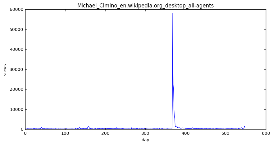
idx = [1, 5, 10, 50, 100, 250,500, 750,1000,1500,2000,3000,4000,5000]
for i in idx:#按词条分类
    plot_entry('en',i)
结果:


npages = 5
top_pages = {}
for key in lang_sets:
    print(key)
    sum_set = pd.DataFrame(lang_sets[key][['Page']])
    sum_set['total'] = lang_sets[key].sum(axis=1)
    sum_set = sum_set.sort_values('total',ascending=False)
    print(sum_set.head(10))
    top_pages[key] = sum
结果:
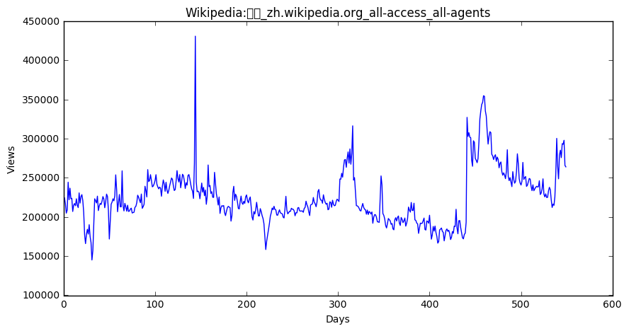
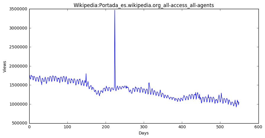
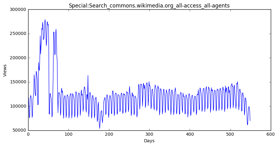
zh
                                                     Page      total
28727   Wikipedia:首页_zh.wikipedia.org_all-access_all-a...  123694312
61350    Wikipedia:首页_zh.wikipedia.org_desktop_all-agents   66435641
105844  Wikipedia:首页_zh.wikipedia.org_mobile-web_all-a...   50887429
28728   Special:搜索_zh.wikipedia.org_all-access_all-agents   48678124
61351      Special:搜索_zh.wikipedia.org_desktop_all-agents   48203843
28089   Running_Man_zh.wikipedia.org_all-access_all-ag...   11485845
30960   Special:链接搜索_zh.wikipedia.org_all-access_all-a...   10320403
63510    Special:链接搜索_zh.wikipedia.org_desktop_all-agents   10320336
60711     Running_Man_zh.wikipedia.org_desktop_all-agents    7968443
30446    瑯琊榜_(電視劇)_zh.wikipedia.org_all-access_all-agents    5891589


fr
                                                     Page      total
27330   Wikipédia:Accueil_principal_fr.wikipedia.org_a...  868480667
55104   Wikipédia:Accueil_principal_fr.wikipedia.org_m...  611302821
7344    Wikipédia:Accueil_principal_fr.wikipedia.org_d...  239589012
27825   Spécial:Recherche_fr.wikipedia.org_all-access_...   95666374
8221    Spécial:Recherche_fr.wikipedia.org_desktop_all...   88448938
26500   Sp?cial:Search_fr.wikipedia.org_all-access_all...   76194568
6978    Sp?cial:Search_fr.wikipedia.org_desktop_all-ag...   76185450
131296  Wikipédia:Accueil_principal_fr.wikipedia.org_a...   63860799
26993   Organisme_de_placement_collectif_en_valeurs_mo...   36647929
7213    Organisme_de_placement_collectif_en_valeurs_mo...   36624145


ru
                                                     Page       total
99322   Заглавная_страница_ru.wikipedia.org_all-access...  1086019452
103123  Заглавная_страница_ru.wikipedia.org_desktop_al...   742880016
17670   Заглавная_страница_ru.wikipedia.org_mobile-web...   327930433
99537   Служебная:Поиск_ru.wikipedia.org_all-access_al...   103764279
103349  Служебная:Поиск_ru.wikipedia.org_desktop_all-a...    98664171
100414  Служебная:Ссылки_сюда_ru.wikipedia.org_all-acc...    25102004
104195  Служебная:Ссылки_сюда_ru.wikipedia.org_desktop...    25058155
97670   Special:Search_ru.wikipedia.org_all-access_all...    24374572
101457  Special:Search_ru.wikipedia.org_desktop_all-ag...    21958472
98301   Служебная:Вход_ru.wikipedia.org_all-access_all...    12162587


ja
                                                     Page      total
120336      メインページ_ja.wikipedia.org_all-access_all-agents  210753795
86431          メインページ_ja.wikipedia.org_desktop_all-agents  134147415
123025       特別:検索_ja.wikipedia.org_all-access_all-agents   70316929
89202           特別:検索_ja.wikipedia.org_desktop_all-agents   69215206
57309       メインページ_ja.wikipedia.org_mobile-web_all-agents   66459122
119609    特別:最近の更新_ja.wikipedia.org_all-access_all-agents   17662791
88897        特別:最近の更新_ja.wikipedia.org_desktop_all-agents   17627621
119625        真田信繁_ja.wikipedia.org_all-access_all-agents   10793039
123292  特別:外部リンク検索_ja.wikipedia.org_all-access_all-agents   10331191
89463      特別:外部リンク検索_ja.wikipedia.org_desktop_all-agents   10327917


es
                                                     Page      total
92205   Wikipedia:Portada_es.wikipedia.org_all-access_...  751492304
95855   Wikipedia:Portada_es.wikipedia.org_mobile-web_...  565077372
90810   Especial:Buscar_es.wikipedia.org_all-access_al...  194491245
71199   Wikipedia:Portada_es.wikipedia.org_desktop_all...  165439354
69939   Especial:Buscar_es.wikipedia.org_desktop_all-a...  160431271
94389   Especial:Buscar_es.wikipedia.org_mobile-web_al...   34059966
90813   Especial:Entrar_es.wikipedia.org_all-access_al...   33983359
143440  Wikipedia:Portada_es.wikipedia.org_all-access_...   31615409
93094   Lali_Espósito_es.wikipedia.org_all-access_all-...   26602688
69942   Especial:Entrar_es.wikipedia.org_desktop_all-a...   25747141


en
                                                    Page        total
38573   Main_Page_en.wikipedia.org_all-access_all-agents  12066181102
9774       Main_Page_en.wikipedia.org_desktop_all-agents   8774497458
74114   Main_Page_en.wikipedia.org_mobile-web_all-agents   3153984882
39180  Special:Search_en.wikipedia.org_all-access_all...   1304079353
10403  Special:Search_en.wikipedia.org_desktop_all-ag...   1011847748
74690  Special:Search_en.wikipedia.org_mobile-web_all...    292162839
39172  Special:Book_en.wikipedia.org_all-access_all-a...    133993144
10399   Special:Book_en.wikipedia.org_desktop_all-agents    133285908
33644       Main_Page_en.wikipedia.org_all-access_spider    129020407
34257  Special:Search_en.wikipedia.org_all-access_spider    124310206


na
                                                    Page     total
45071  Special:Search_commons.wikimedia.org_all-acces...  67150638
81665  Special:Search_commons.wikimedia.org_desktop_a...  63349756
45056  Special:CreateAccount_commons.wikimedia.org_al...  53795386
45028  Main_Page_commons.wikimedia.org_all-access_all...  52732292
81644  Special:CreateAccount_commons.wikimedia.org_de...  48061029
81610  Main_Page_commons.wikimedia.org_desktop_all-ag...  39160923
46078  Special:RecentChangesLinked_commons.wikimedia....  28306336
45078  Special:UploadWizard_commons.wikimedia.org_all...  23733805
81671  Special:UploadWizard_commons.wikimedia.org_des...  22008544
82680  Special:RecentChangesLinked_commons.wikimedia....  21915202


de
                                                     Page       total
139119  Wikipedia:Hauptseite_de.wikipedia.org_all-acce...  1603934248
116196  Wikipedia:Hauptseite_de.wikipedia.org_mobile-w...  1112689084
67049   Wikipedia:Hauptseite_de.wikipedia.org_desktop_...   426992426
140151  Spezial:Suche_de.wikipedia.org_all-access_all-...   223425944
66736   Spezial:Suche_de.wikipedia.org_desktop_all-agents   219636761
140147  Spezial:Anmelden_de.wikipedia.org_all-access_a...    40291806
138800  Special:Search_de.wikipedia.org_all-access_all...    39881543
68104   Spezial:Anmelden_de.wikipedia.org_desktop_all-...    35355226
68511   Special:MyPage/toolserverhelferleinconfig.js_d...    32584955
137765  Hauptseite_de.wikipedia.org_all-access_all-agents    31732458
for key in top_pages:
    fig = plt.figure(1,figsize=(10,5))
    cols = train.columns
    cols = cols[1:-1]
    data = train.loc[top_pages[key],cols]
    plt.plot(days,data)
    plt.xlabel('Days')
    plt.ylabel('Views')
    plt.title(train.loc[top_pages[key],'Page'])
    plt.show()
结果:


 浙公网安备 33010602011771号