python可视化_matplotlib

Posted on 2019-08-24 08:46 天戈朱阅读(1221) 评论(0) 编辑收藏举报

对于Python数据可视化库，matplotlib 已经成为事实上的数据可视化方面最主要的库，此外还有很多其他库，例如vispy，bokeh， seaborn，pyga，folium 和 networkx，这些库有些是构建在 matplotlib 之上，还有些有其他一些功能。

matplotlib
基本函数
中文乱码
plot：线性图
bar：柱状图
barh：水平柱状图
pie：饼图
scatter：散点图
hist：直方图
stackplot：面积图
subplot：子图布局
GridSpec：网格布局

matplotlib

matplotlib 是一个基于 Python 的 2D 绘图库，其可以在跨平台的在各种硬拷贝格式和交互式环境中绘制出高图形。Matplotlib 能够创建多数类型的图表，如条形图，散点图，条形图，饼图，堆叠图，3D 图和地图图表。

％matplotlib 命令可以在当前的 Notebook 中启用绘图。Matlibplot 提供了多种绘图 UI ，可进行如下分类：

弹出窗口和交互界面：％matplotlib qt 和％matplot tk
非交互式内联绘图：％matplotlib inline
交互式内联绘图：％matplotlib notebook－－＞别用这个，它会让开关变得困难。

安装Matplotlib命令：pip install matplotlib

基本函数

legend：增加图例（线的标题），格式：plt.legend(handles=(line1, line2, line3),labels=('label1', 'label2', 'label3'),loc='upper right'), 见如下示例代码

1 ln1, = plt.plot(x_data, y_data, color = 'red', linewidth = 2.0, linestyle = '--')
2 ln2, = plt.plot(x_data, y_data2, color = 'blue', linewidth = 3.0, linestyle = '-.')
3 plt.legend(handles=[ln2, ln1], labels=['Android基础', 'Java基础'],  loc='lower right')

loc参数值：

'best'：自动选择最佳位置
'upper right'：将图例放在右上角。
'upper left'：将图例放在左上角。
'lower left'：将图例放在左下角。
'lower right'：将图例放在右下角。
'right'：将图例放在右边。
'center left'：将图例放在左边居中的位置。
'center right'：将图例放在右边居中的位置。
'lower center'：将图例放在底部居中的位置。
'upper center'：将图例放在顶部居中的位置。
'center'：将图例放在中心。

figure：新建一个画布，格式：figure(num=None, figsize=None, dpi=None, facecolor=None, edgecolor=None, frameon=True)

num：图像编号或名称，数字为编号，字符串为名称
figsize：指定figure的宽和高，单位为英寸；
dpi：指定绘图对象的分辨率，即每英寸多少个像素，缺省值为80；1英寸等于2.5cm,A4纸是 21*30cm的纸张
frameon：是否显示边框

spines：在matplotlib的图中，默认有四个轴，两个横轴和两个竖轴，可以通过ax = plt.gca()方法获取，gca是‘get current axes’的缩写，获取图像的轴，总共有四个轴 top、bottom、left、right

axis指定要用的轴：由于axes会获取到四个轴，而我们只需要两个轴，所以我们需要把另外两个轴隐藏，把顶部和右边轴的颜色设置为none, 如：plt.gca().spines['top'].set_color('none')
移动轴到指定位置：ax.spines[‘bottom’]获取底部的轴，通过 set_position 方法，设置底部轴的位置，例如：ax.spines[‘bottom’].set_position((‘data’,0)) 表示设置底部轴移动到竖轴的0坐标位置，设置轴设置的方法相同

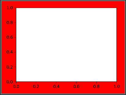
示例代码：

1 import matplotlib.pyplot as plt
2 
3 fig = plt.figure(figsize=(4, 3), frameon=True, facecolor='r')
4 ax = fig.add_subplot(1, 1, 1)
5 ax.spines['top'].set_color = 'none'
6 ax.spines['right'].set_color = 'none'
7 ax.spines['left'].set_position(('data', 0))
8 ax.spines['bottom'].set_position(('data', 0))
9 plt.show()

View Code

效果图：

中文乱码

问题描述：matplotlib绘制图像在显示中文时候，中文会变成小方格子。其实plotlib是支持中文编码的，造成这个现象的原因是，matplotlib库的配置信息里面没有中文字体的相关信息
解决方案：在python脚本中动态设置 matplotlibrc，这样就避免了更改配置文件的麻烦，方便灵活，更改了字体导致显示不出负号，将配署文件中 axes.unicode minus :True 修改为 Falsest 就可以了，代码如下：

1 from pylab import mpl
2 
3 mpl.rcParams['font.sans-serif'] = 'FangSong' # 指定默认字体
4 mpl.rcParams['axes.unicode_minus'] = False  # 解决保存图像是负号'-'显示为方块的问题

Windows的字体对应名称如下

黑体：SimHei
微软雅黑：Microsoft YaHei
微软正黑体：Microsoft JhengHei
新宋体：NSimSun
新细明体：PMingLiU
标楷体：DFKai-SB
仿宋：FangSong
楷体：KaiTi
仿宋_GB2312： FangSong_GB2312
楷体_GB2312： KaiTi_GB2312

plot：线性图

格式：plt.plot(x,y,format_string,**kwargs)

x轴数据，y轴数据，format_string控制曲线的格式字串
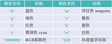
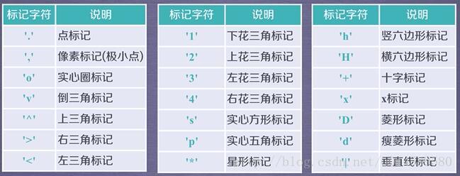
format_string：由颜色字符，风格字符，和标记字符。具体形式 fmt = '[color][marker][line]' ，fmt接收的是每个属性的单个字母缩写，见如下代码：
1. plot(x,y2,color='green', marker='o', linestyle='dashed', linewidth=1, markersize=6)
2. plot(x,y3,color='#900302',marker='+',linestyle='-')
3. 还可包含有其它的属性，如：markerfacecolor：标记颜色、markersize：标记大小等等

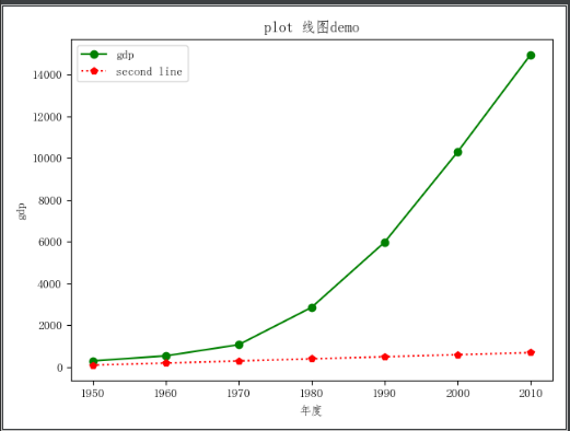
示例：

 1 import matplotlib.pyplot as plt
 2 from pylab import mpl
 3 
 4 mpl.rcParams['font.sans-serif'] = 'FangSong' # 指定默认字体
 5 mpl.rcParams['axes.unicode_minus'] = False  # 解决保存图像是负号'-'显示为方块的问题
 6 
 7 year = ['1950', '1960', '1970', '1980', '1990', '2000', '2010']
 8 gdp = [300.2, 543.3, 1075.9, 2862.5, 5979.6, 10298.7, 14958.3]
 9 y_data = [100, 200, 300, 400, 500, 600, 700]
10 
11 
12 def draw_plot():
13     # plt.plot(year, gdp, 'go-', year, y_data, 'rp:')
14     plt.plot(year, gdp, 'go-', label='gdp')
15     plt.plot(year, y_data, 'rp:', label='second line')
16     plt.title("plot 线图demo")
17     plt.xlabel('年度')
18     plt.ylabel('gdp')
19     plt.legend()  #生成默认图例
20     plt.show()

View Code

效果图：

bar：柱状图

格式：bar(left, height, width, alpha=1, width=0.8, color=, edgecolor=, label=, lw=3)

left：x轴的位置序列，一般采用arange函数产生一个序列；
height：y轴的数值序列，也就是柱形图的高度，一般就是我们需要展示的数据；
width：柱形图的宽度，一般这是为1即可；
alpha：透明度
width：为柱形图的宽度，一般这是为0.8即可；
color或facecolor：柱形图填充的颜色；
edgecolor：图形边缘颜色
label：解释每个图像代表的含义
linewidth or linewidths or lw：边缘or线的宽度

示例

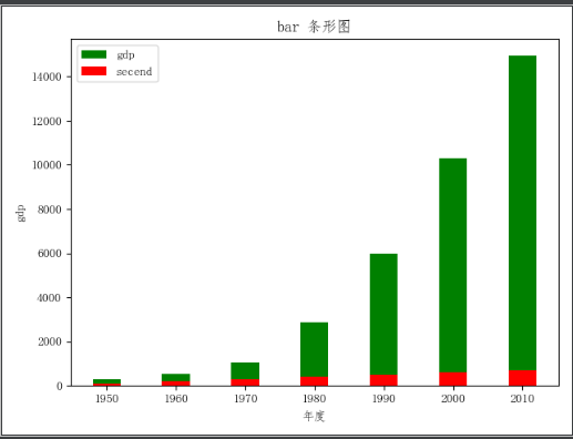
 1 def draw_bar():
 2     plt.bar(x=year, height=gdp, width=0.4, label='gdp', color='green')
 3     plt.bar(x=year, height=y_data, width=0.4, label='secend', color='red')
 4     # 在柱状图上显示具体数值, ha参数控制水平对齐方式, va控制垂直对齐方式
 5     for x, y in enumerate(y_data):
 6         plt.text(x, y - 400, '%s' % y, ha='center', va='bottom')
 7     for x, y in enumerate(gdp):
 8         plt.text(x, y + 400, '%s' % y, ha='center', va='top')
 9 
10     plt.title("bar 条形图")
11     plt.xlabel('年度')
12     plt.ylabel('gdp')
13     plt.legend()
14     plt.show()

View Code

效果图：

使用 bar() 函数绘制柱状图时，默认不会在柱状图上显示具体的数值。为了能在柱状图上显示具体的数值，程序可以调用 text() 函数在数据图上输出文字，增加如下代码：1for x, y in enumerate(y_data):

1     for x, y in enumerate(y_data):
2         plt.text(x, y - 400, '%s' % y, ha='center', va='bottom')
3     for x, y in enumerate(gdp):
4         plt.text(x, y + 400, '%s' % y, ha='center', va='top')

在使用 text() 函数输出文字时，该函数的前两个参数控制输出文字的 X、Y 坐标，第三个参数则控制输出的内容。其中 va 参数控制文字的垂直对齐方式，ha 参数控制文字的水平对齐方式。
对于上面的代码，由于 X 轴数据是一个字符串列表，因此 X 轴实际上是以列表元素的索引作为刻度值的。因此，当程序指定输出文字的 X 坐标为 0 时，表明将该文字输出到第一个条柱处；对于 Y 坐标而言，条柱的数值正好在条柱高度所在处，如果指定 Y 坐标为条柱的数值 +400，就是控制将文字输出到条柱略上一点的位置。

效果图：

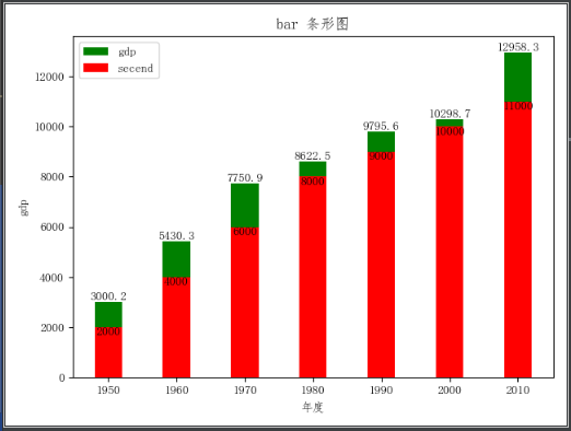
如上图所示的显示效果来看柱状图重叠，为了实现条柱井列显示的效果，首先分析条柱重叠在一起的原因。使用 Matplotlib 绘制柱状图时同样也需要 X 轴数据，本程序的 X 轴数据是元素为字符串的 list 列表，因此程序实际上使用各字符串的索引作为 X 轴数据。比如 '1950' 字符串位于列表的第一个位置，因此代表该条柱的数据就被绘制在 X 轴的刻度值1处（由于两个柱状图使用了相同的 X 轴数据，因此它们的条柱完全重合在一起）。为了将多个柱状图的条柱并列显示，程序需要为这些柱状图重新计算不同的 X 轴数据。为了精确控制条柱的宽度，程序可以在调用 bar() 函数时传入 width 参数，这样可以更好地计算条柱的并列方式。

示例：

 1 def draw_bar2():
 2     barwidth=0.4
 3     plt.bar(x=range(len(year)), height=gdp, width=0.4, label='gdp', color='green')
 4     plt.bar(x=np.arange(len(year)) + barwidth, height=y_data, width=0.4, label='secend', color='red')
 5     # 在柱状图上显示具体数值, ha参数控制水平对齐方式, va控制垂直对齐方式
 6     for x, y in enumerate(gdp):
 7         plt.text(x, y + 400, '%s' % y, ha='center', va='top')
 8     for x, y in enumerate(y_data):
 9         plt.text(x + barwidth, y + 400, '%s' % y, ha='center', va='top')
10 
11     plt.title("bar 条形图")
12     plt.xlabel('年度')
13     plt.ylabel('gdp')
14     plt.legend()
15     plt.show()

View Code

效果图：

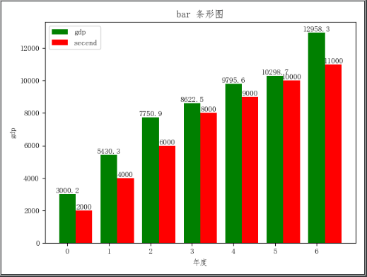
运行上面程序，将会发现该柱状图的 X 轴的刻度值变成 0、1、2 等值，不再显示年份。为了让柱状图的 X 轴的刻度值显示年份，程序可以调用 xticks() 函数重新设置 X 轴的刻度值，如下：

plt.xticks(np.arange(len(year)) + barwidth/2, year)
bar_width/2：这些刻度值将被恰好添加在两个条柱之间

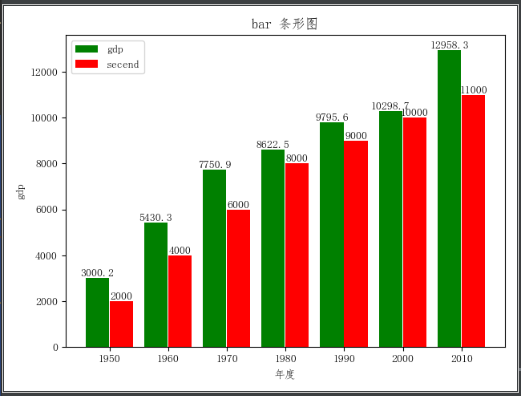
希望两个条柱之间有一点缝隙，那么程序只要对第二个条柱的 X 轴数据略做修改即可，完整代码如下：

 1 def draw_bar2():
 2     barwidth=0.4
 3     plt.bar(x=range(len(year)), height=gdp, width=barwidth, label='gdp', color='green')
 4     plt.bar(x=np.arange(len(year)) + barwidth + 0.01, height=y_data, width=barwidth, label='secend', color='red')
 5     # 在柱状图上显示具体数值, ha参数控制水平对齐方式, va控制垂直对齐方式
 6     for x, y in enumerate(gdp):
 7         plt.text(x, y + 400, '%s' % y, ha='center', va='top')
 8     for x, y in enumerate(y_data):
 9         plt.text(x + barwidth + 0.01, y + 400, '%s' % y, ha='center', va='top')
10 
11     #X轴添加刻度
12     plt.xticks(np.arange(len(year)) + barwidth/2 + 0.01, year)
13     plt.title("bar 条形图")
14     plt.xlabel('年度')
15     plt.ylabel('gdp')
16     plt.legend()
17     plt.show()

View Code

效果图：

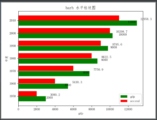
barh：水平柱状图

barh() 函数的用法与 bar() 函数的用法基本一样，只是在调用 barh() 函数时使用 y参数传入 Y 轴数据，使用 width 参数传入代表条柱宽度的数据。

示例:

 1 def draw_barh():
 2     barwidth = 0.4
 3     plt.barh(y=range(len(year)), width=gdp, height=barwidth, label='gdp', color='green')
 4     plt.barh(y=np.arange(len(year)) + barwidth + 0.01, width=y_data, height=barwidth, label='secend', color='red')
 5     # 在柱状图上显示具体数值, ha参数控制水平对齐方式, va控制垂直对齐方式
 6     for y, x in enumerate(gdp):
 7         plt.text(x + 1000, y + barwidth/2, '%s' % x, ha='center', va='bottom')
 8     for y, x in enumerate(y_data):
 9         plt.text(x + 1400, y + barwidth/2 - 0.01, '%s' % x, ha='center', va='top')
10 
11     # y轴添加刻度
12     plt.yticks(np.arange(len(year)) + barwidth / 2 + 0.01, year)
13     plt.title("barh 水平柱状图")
14     plt.xlabel('gdp')
15     plt.ylabel('年度')
16     plt.legend()
17     plt.show()

View Code

效果图：

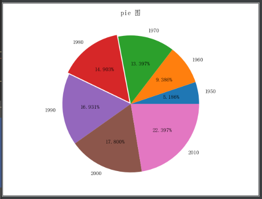
pie：饼图

格式：pie(x, explode=None, labels=None, colors=('b', 'g', 'r', 'c', 'm', 'y', 'k', 'w'), autopct=None, pctdistance=0.6, shadow=False, labeldistance=1.1, startangle=None, radius=None, counterclock=True, wedgeprops=None, textprops=None, center = (0, 0), frame = False )

创建饼图最重要的两个参数就是 x 和 labels，其中 x 指定饼图各部分的数值，labels 则指定各部分对应的标签
通常，饼图用于显示部分对于整体的情况，通常以％为单位。幸运的是，Matplotlib 会处理切片大小以及一切事情，我们只需要提供数值。
x：绘图数据
explode：突出显示，如将第4个数据显示：explode = [0, 0, 0, 0.3, 0, 0, 0, 0, 0, 0, 0]
labels：显示标签
autopct：设置百分比的格式，如保留3位小数：autopct='%.3f%%'
pctdistance：置百分比标签与圆心的距离，如：pctdistance=0.8
labeldistance：设置标签与圆心的距离，如：startangle = 180
startangle：设置饼图的初始角度，如：startangle = 180
center ：设置饼图的圆心（相当于X轴和Y轴的范围）,如：center = (4, 4)
radius ：设置饼图的半径（相当于X轴和Y轴的范围），如：radius = 3.8
counterclock ：是否逆时针，如这里设置为顺时针方向：counterclock = False,
wedgeprops：设置饼图内外边界的属性值，如：wedgeprops = {'linewidth': 1, 'edgecolor':'green'}
textprops：设置文本标签的属性值，如：textprops = {'fontsize':12, 'color':'black'}
frame ：是否显示饼图的圆圈，如此处设为显示：frame = 1

示例

1 def draw_pie():
2     plt.pie(x=gdp,
3             labels=year,
4             autopct='%.3f%%',
5             explode=[0, 0, 0, 0.03, 0, 0, 0])
6 
7     plt.title("pie 图")
8     plt.show()

View Code

效果：

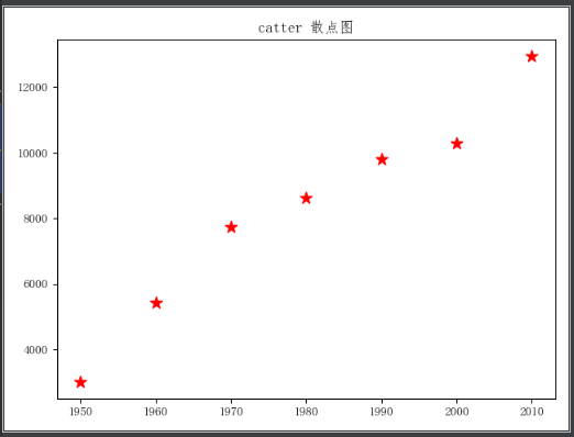
scatter：散点图

格式：scatter(x, y, s=None, c=None, marker=None, cmap=None, norm=None, vmin=None, vmax=None, alpha=None, linewidths=None, verts=None, edgecolors=None, hold=None, data=None, **kwargs)

x, y：指 x 轴、y轴数据
s：指定散点的大小（设置点半径），如：s=50
c：指定散点的颜色。如：c='red'
alpha：指定散点的透明度。如：alpha = 0.5
marker：指定散点的图形样式，见最上面标记字符图，如：marker='p'

示例：

1 def draw_catter():
2     plt.scatter(x=year, y=gdp, c='red', marker='*', s=100)
3 
4     plt.title("catter 散点图")
5     plt.show()

View Code

效果：

hist：直方图

柱状图与直方图：

柱状图是用条形的长度表示各类别频数的多少，其宽度（表示类别）则是固定的；
直方图是用面积表示各组频数的多少，矩形的高度表示每一组的频数或频率，宽度则表示各组的组距，因此其高度与宽度均有意义。
由于分组数据具有连续性，柱状图的各矩形通常是连续排列，而条形图则是分开排列。
柱状图主要用于展示分类数据，而直方图则主要用于展示数据型数据

格式：pyplot.hist(x, bins=None, range=None, normed=False, weights=None, cumulative=False, bottom=None, histtype=’bar’, align=’mid’, orientation=’vertical’, rwidth=None, log=False, color=None, label=None, stacked=False, hold=None, data=None, **kwargs)

x：指定每个bin(箱子)分布的数据,对应x轴
bins : 这个参数指定bin(箱子)的个数,也就是总共有几条条状图
normed : 是否将得到的直方图向量归一化
histtype : {‘bar’, ‘barstacked’, ‘step’, ‘stepfilled’}

函数返回值：

n : array or list of arrays(箱子的值)
bins : array(箱子的边界)
patches : list or list of lists

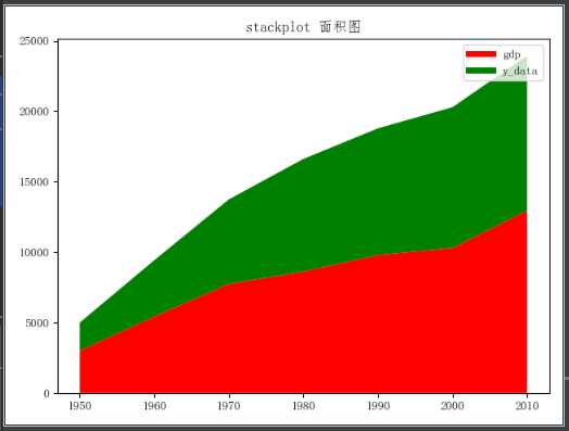
stackplot：面积图

格式：stackplot(x, *args, labels=(), colors=None, baseline='zero', data=None, **kwargs)

示例：

1  plt.stackplot(year, gdp, y_data, colors=['r', 'g'])  
2     plt.title("stackplot 面积图")
3     plt.show()

效果：

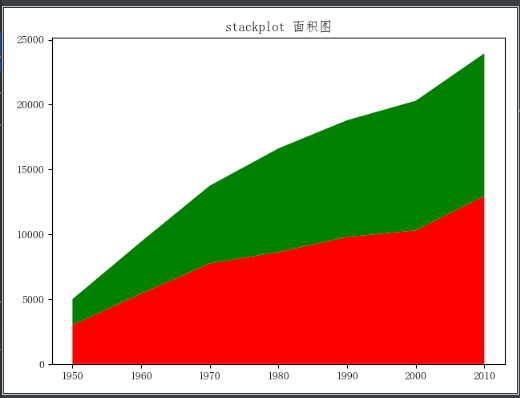
从图上看不出颜色代表的含义，增加图例，完整代码如下：

1 def draw_stackplot():
2     plt.plot([], [], color='r', label='gdp', linewidth=5)
3     plt.plot([], [], color='g', label='y_data', linewidth=5)
4     plt.stackplot(year, gdp, y_data, colors=['r', 'g'])
5     plt.title("stackplot 面积图")
6     plt.legend()
7     plt.show()

View Code

效果图：

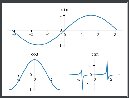
subplot：子图布局

subplot 在一张数据图上包含多个子图，格式：subplot(nrows, ncols, index, **kwargs)

nrows：指定将数据图区域分成多少行；
ncols：指定将数据图区域分成多少列；
index：指定获取第几个区域

subplot() 函数也支持直接传入一个三位数的参数，其中第一位数将作为 nrows 参数；第二位数将作为 ncols 参数；第三位数将作为 index 参数。

示例：

 1 def draw_subplot():
 2     plt.figure(figsize=(4, 3))
 3 
 4     x_data = np.linspace(-np.pi, np.pi, 64, endpoint=True)
 5     plt.subplot(2, 1, 1)
 6     plt.plot(x_data, np.sin(x_data))
 7     plt.gca().spines['top'].set_color('none')
 8     plt.gca().spines['right'].set_color('none')
 9     plt.gca().spines['left'].set_position(('data', 0))
10     plt.gca().spines['bottom'].set_position(('data', 0))
11     plt.title('sin')
12 
13     plt.subplot(2, 2, 3)
14     plt.plot(x_data, np.cos(x_data))
15     plt.gca().spines['top'].set_color('none')
16     plt.gca().spines['right'].set_color('none')
17     plt.gca().spines['left'].set_position(('data', 0))
18     plt.gca().spines['bottom'].set_position(('data', 0))
19     plt.title('cos')
20 
21     plt.subplot(2, 2, 4)
22     plt.plot(x_data, np.tan(x_data))
23     plt.gca().spines['top'].set_color('none')
24     plt.gca().spines['right'].set_color('none')
25     plt.gca().spines['left'].set_position(('data', 0))
26     plt.gca().spines['bottom'].set_position(('data', 0))
27     plt.title('tan')
28 
29     plt.show()

View Code

效果：

GridSpec：网格布局

指定在给定GridSpec中的子图位置

示例：

 1 def draw_gridspace():
 2     plt.figure(figsize=(4, 3))
 3 
 4     x_data = np.linspace(-np.pi, np.pi, 64, endpoint=True)
 5     gs = gridspace.GridSpec(2, 2)
 6     ax1 = plt.subplot(gs[0, :])
 7     ax2 = plt.subplot(gs[1, 0])
 8     ax3 = plt.subplot(gs[1, 1])
 9 
10     ax1.plot(x_data, np.sin(x_data))
11     ax1.spines['top'].set_color('none')
12     ax1.spines['right'].set_color('none')
13     ax1.spines['left'].set_position(('data', 0))
14     ax1.spines['bottom'].set_position(('data', 0))
15     ax1.set_title('sin')
16 
17     ax2.plot(x_data, np.cos(x_data))
18     ax2.spines['top'].set_color('none')
19     ax2.spines['right'].set_color('none')
20     ax2.spines['left'].set_position(('data', 0))
21     ax2.spines['bottom'].set_position(('data', 0))
22     ax2.set_title('cos')
23 
24     ax3.plot(x_data, np.tan(x_data))
25     ax3.spines['top'].set_color('none')
26     ax3.spines['right'].set_color('none')
27     ax3.spines['left'].set_position(('data', 0))
28     ax3.spines['bottom'].set_position(('data', 0))
29     ax3.set_title('tan')
30 
31     plt.show()

View Code

效果与上节 subplot 一致

参考资料

会员力量，点亮园子希望

刷新页面返回顶部

天戈朱

公告

python可视化_matplotlib