Python用Keras的LSTM神经网络进行时间序列预测天然气价格例子

原文链接：http://tecdat.cn?p=26519 

原文出处：拓端数据部落公众号

 

一个简单的编码器-解码器LSTM神经网络应用于时间序列预测问题：预测天然气价格，预测范围为 10 天。“进入”时间步长也设置为 10 天。) 只需要 10 天来推断接下来的 10 天。可以使用 10 天的历史数据集以在线学习的方式重新训练网络。

数据集是 天然气价格 ，具有以下功能：

• 日期（从 1997 年到 2020 年）- 为 每天数据
• 以元计的天然气价格

读取数据并将日期作为索引处理

1.  
    
2.  
   # 固定日期时间并设置为索引
3.  
   dftet.index = pd.DatetimeIndex
4.  
    
5.  
   # 用NaN来填补缺失的日期（以后再补）
6.  
   dargt = f_arget.reindex(ales, fill_value=np.nan)
7.  
    
8.  
   # 检查
9.  
   print(d_tret.dtypes)
10.  
    df_aget.head(10)

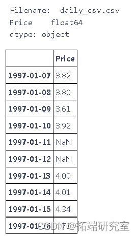
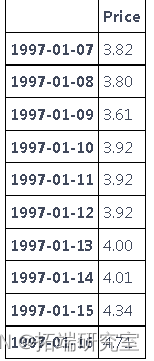
处理缺失的日期

1.  
   # 数据归纳（，使用 "向前填充"--根据之前的值进行填充）。
2.  
   dfaet.fillna(method='ffill', inplace=True)

特征工程

因为我们正在使用深度学习，所以特征工程将是最小的。

• One-hot 编码“is_weekend”和星期几
• 添加行的最小值和最大值（可选）

通过设置固定的上限（例如 30 倍中位数）修复异常高的值

1.  
    
2.  
    
3.  
   # 在df_agg中修复任何非常高的值 - 归一化为中值
4.  
   for col in co_to_fi_ies:
5.  
   dgt[col] = fixnaes(dftget[col])

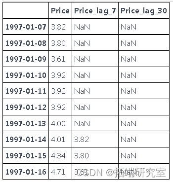
添加滞后

1.  
    
2.  
   # 增加每周的滞后性
3.  
   df_tret = addag(d_aget, tare_arble='Price', step_ak=7)
4.  
   # Add 30 day lag
5.  
   df_get = ad_ag(df_ret, tagt_able='Price', sep_bck=30)

1.  
   # 合并后删除任何有NA值的列
2.  
   d_gt.dropna(inplace=True)
3.  
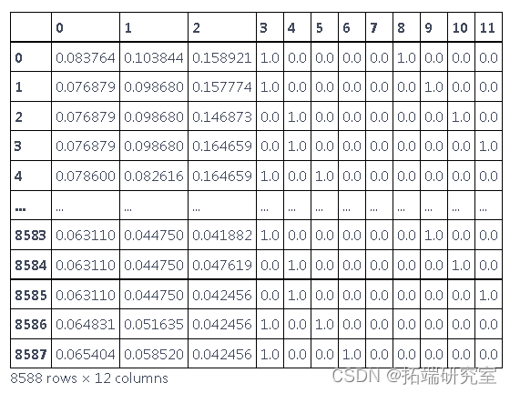
   print(dfget.shape)
4.  
    
5.  
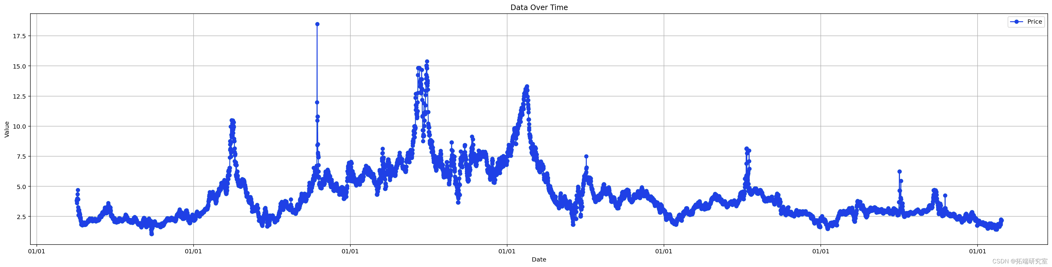
   tie_nx = df_art.index

归一化

• 归一化或最小-最大尺度（需要减小较宽的数值范围，以便 LSTM 收敛）。

1.  
   # 标准化训练数据[0, 1]
2.  
   sclr = prcsing.Maxcaer((0,1))

准备训练数据集

• 时间步数 = 1
• 时间步数 = nsteout小时数（预测范围）

在这里，我们将数据集从 [samples, features] 转换为 [samples, steps, features] - 与算法 LSTM 一起使用的形状。下面的序列拆分使用“walk-forward”方法来创建训练数据集。

1.  
   # 多变量多步骤编码器-解码器 lstm 示例
2.  
   # 选择一个时间步骤的数量
3.  
    
4.  
    
5.  
    
6.  
   # 维度变成[样本数、步骤、特征]
7.  
   X, y = splices(datasformed, n_ep_in, n_ep_out)
8.  
    
9.  
   # 分成训练/测试
10.  
    et_ut = int(0.05*X.shpe[0])
11.  
    X_tain, X_est, ytrain, y_tst = X[:-tetaont], X[-tes_ont:], y[:-tstmunt], y[-es_unt:]

训练模型

这利用了长期短期记忆算法。

1.  
   # 实例化和训练模型
2.  
   print
3.  
   model = cre_odel(n_tps_in, n_tep_out, n_feures, lerig_rate=0.0001)

 

探索预测

1.  
   %%time
2.  
   #加载特定的模型
3.  
    
4.  
   model = lod_id_del(
5.  
   n_stepin,
6.  
   n_sep_out,
7.  
   X_tan.shape[2])

1.  
   # 展示对一个样本的预测
2.  
   testle_ix = 0
3.  
   yat = mdel.predict(X_tet[est_amle_ix].reshape((1,n_sep_in, nfatues)),erbose=Tue)

1.  
   # 计算这一个测试样本的均方根误差
2.  
   rmse = math.sqrt

plot_result(yhat[0], scaler, saved_columns)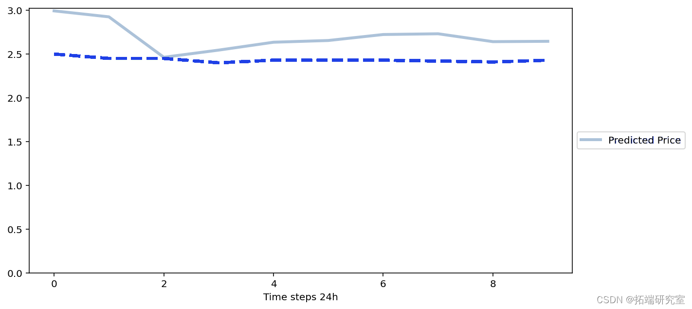

平均 RMSE

1.  
   # 收集所有的测试RMSE值
2.  
   rmesores = []
3.  
   for i in range:
4.  
   yhat = oel.predict(Xtet[i].reshape((1, _stes_in, _faues)), verbose=False)
5.  
   # 计算这一个测试样本的均方根误差
6.  
   rmse = math.sqrt(mensqaerror(yhat[0], y_test[i]))

训练整个数据集

1.  
   #在所有数据上实例化和训练模型
2.  
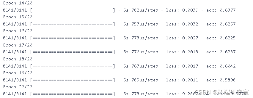
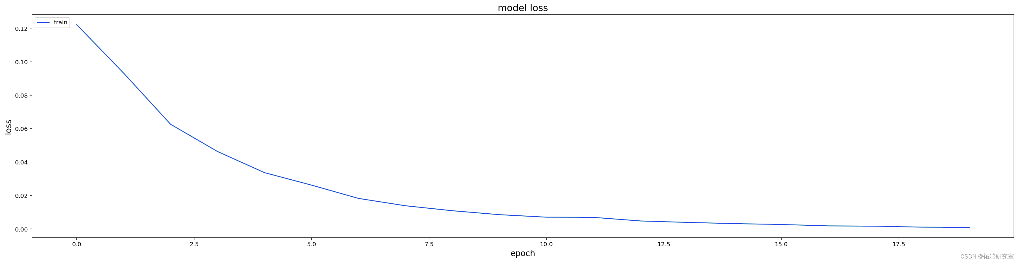
   modl_l = cret_mel(nsep_in, steps_ou, n_etures,learnnrate=0.0001)
3.  
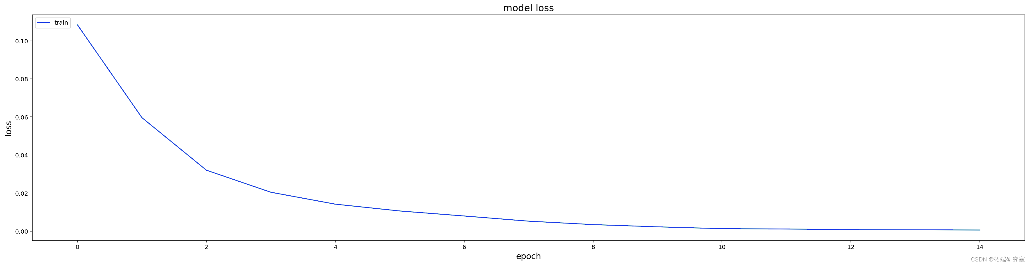
   mde_all, ru_ime, weighfie = trin(md_all, X, y, batcsie=16, neohs=15)

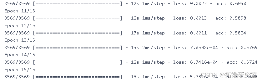
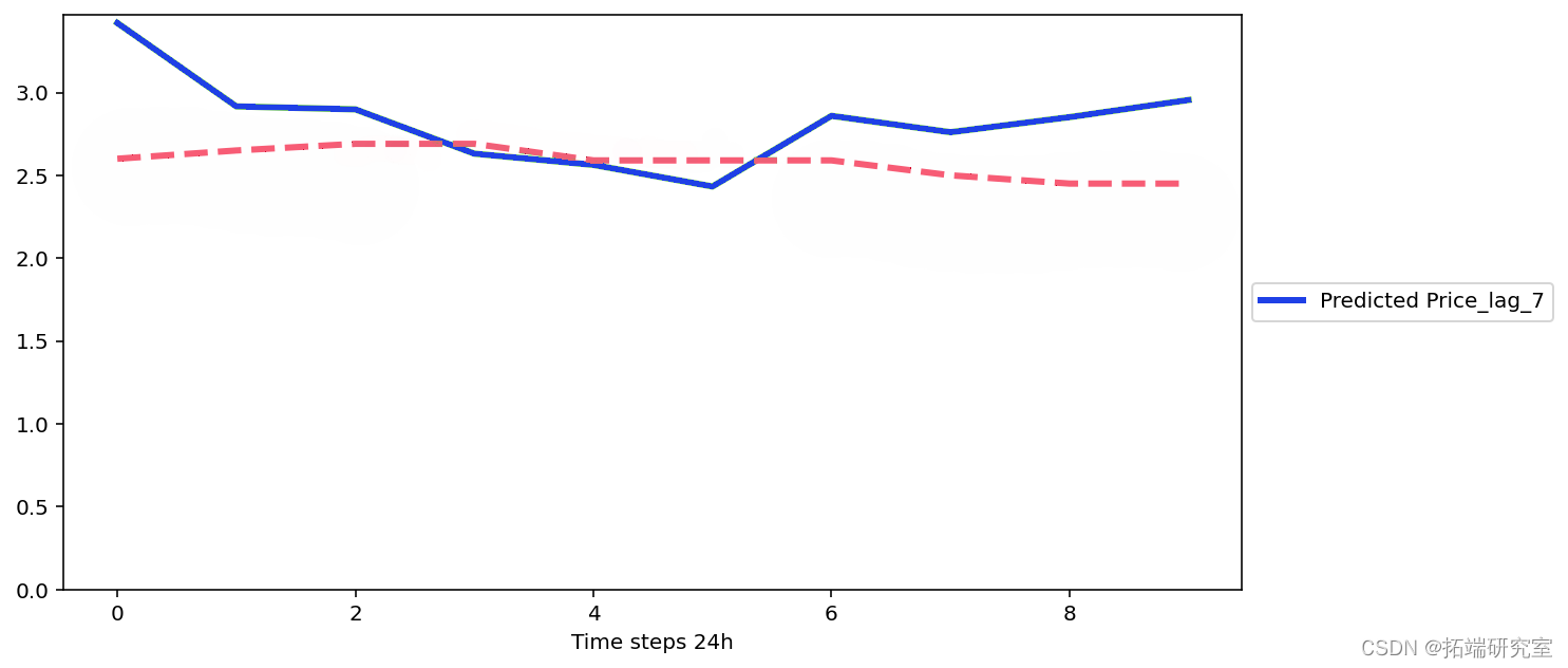
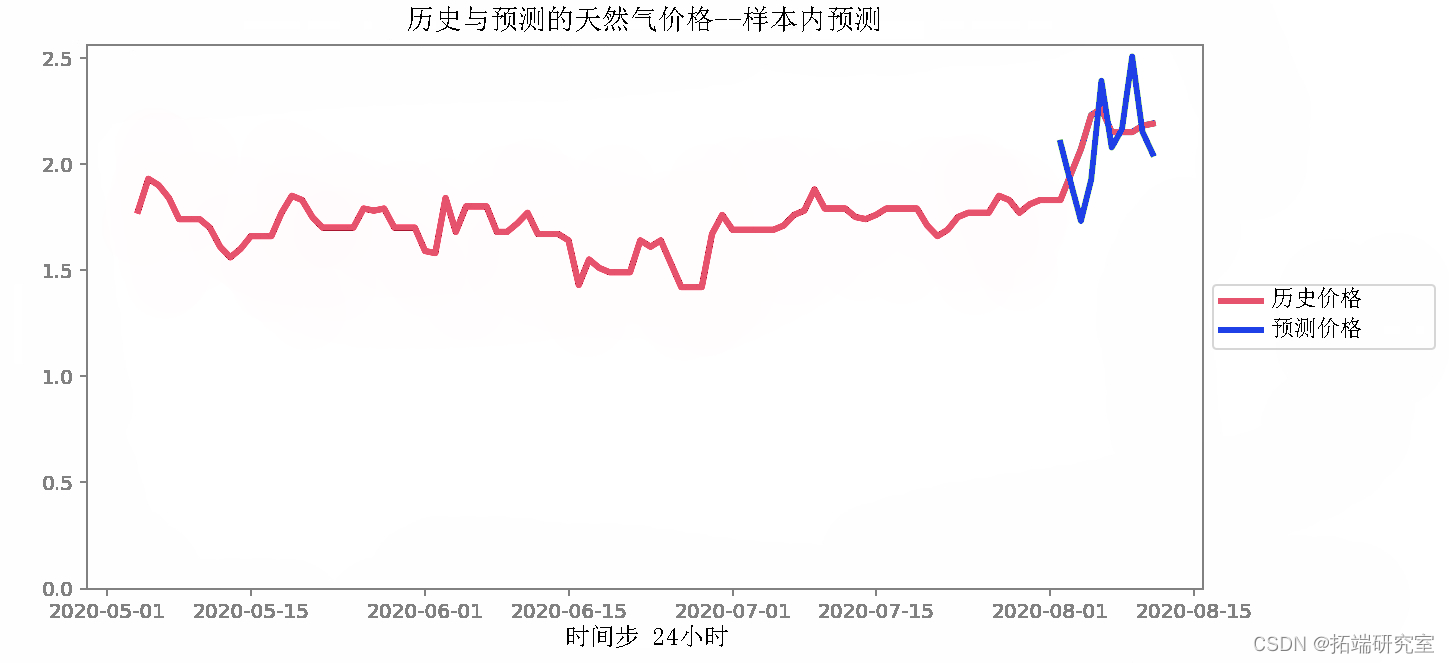
​​​​​​​样本内预测

注意：模型已经“看到”或训练了这些样本，但我们希望确保它与预测一致。如果它做得不好，模型可能会欠拟合或过拟合。要尝试的事情：

• 增加或减少批量大小
• 增加或减少学习率
• 更改网络中 LSTM 的隐藏层数

1.  
    
2.  
   # 获得10个步
3.  
   da_cent = dfret.iloc[-(ntes_in*2):-nsps_in]
4.  
    
5.  
   # 标准化
6.  
   dta_ectormed = sclr.rasfrm(daareent)
7.  
    
8.  
   # 维度变成[样本数、步骤、特征]
9.  
   n_res = dtcentorm.shape[1]
10.  
    X_st = data_recn_trsrd.reshape((1, n_tps_n, n_feares))
11.  
     
12.  
    # 预测
13.  
    foecst = mlll.predict(X_past)
14.  
     
15.  
    # 扩大规模并转换为DF
16.  
    forcast = forast.resape(n_eaturs))
17.  
    foect = saer.inese_transform(forecast)
18.  
    fuure_dtes df_targe.ide[-n_steps_out:]
19.  
     
20.  
    # 绘图
21.  
    histrcl = d_aet.ioc[-100:, :1] # 获得历史数据的X步回溯
22.  
    for i in ane(oisae[1]):
23.  
    fig = plt.igre(fgze=(10,5))
24.  
     
25.  
    # 绘制df_agg历史数据
26.  
    plt.plot(.iloc[:,i]
27.  
     
28.  
    # 绘制预测图
29.  
    plt.plot(frc.iloc[:,i])
30.  
     
31.  
    # 标签和图例
32.  
    plt.xlabel

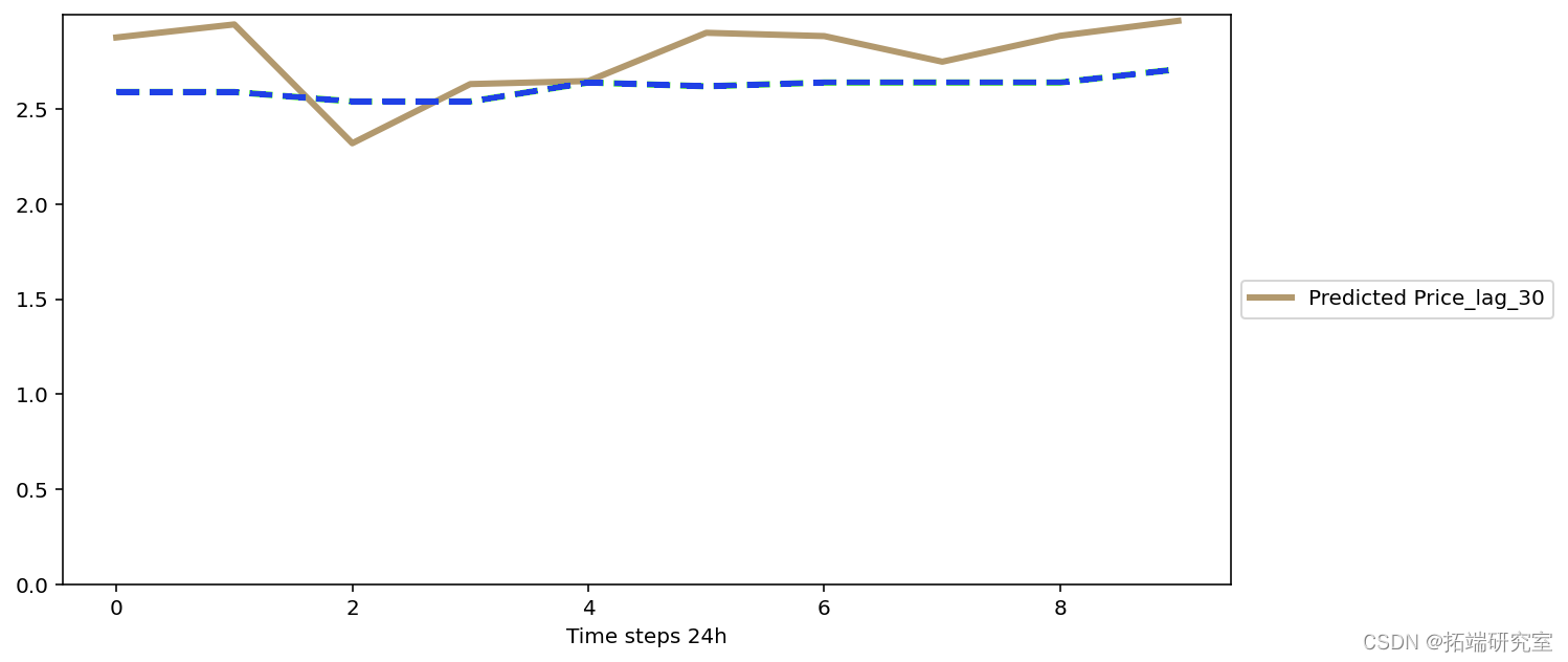
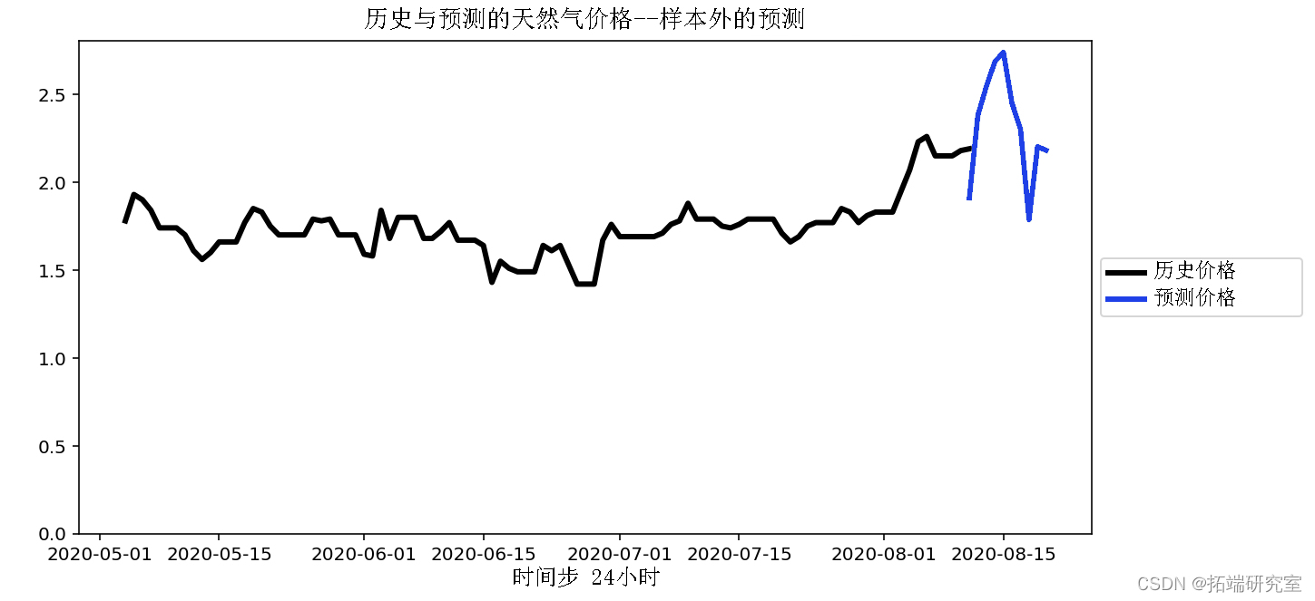
预测样本外

1.  
    
2.  
   # 获取最后10步
3.  
   dtareent = dfargt.iloc[-nstpsin:]。
4.  
    
5.  
   # 缩放
6.  
   dta_ecntranfomed = scaler.trasorm(data_recent)
7.  
    
8.  
    
9.  
   # 预测
10.  
    forct = meall.rict(_past)
11.  
     
12.  
    # 扩大规模并转换为DF
13.  
    foreast = foecs.eshape(_seps_ut, n_eatures))
14.  
    foreast = sclerinvers_tranorm(focast)
15.  
    futur_daes = pd.daternge(df_argetinex[-1], priods=step_out, freq='D')
16.  
     
17.  
     
18.  
    # 绘图
19.  
    htrical = df_taet.iloc[-100:, :1] # 获得历史数据的X步回溯
20.  
    # 绘制预测图
21.  
    plt.plot(fectoc[:,i])
22.  
     

---

最受欢迎的见解

1.在python中使用lstm和pytorch进行时间序列预测

2.python中利用长短期记忆模型lstm进行时间序列预测分析

3.使用r语言进行时间序列（arima，指数平滑）分析

4.r语言多元copula-garch-模型时间序列预测

5.r语言copulas和金融时间序列案例

6.使用r语言随机波动模型sv处理时间序列中的随机波动

7.r语言时间序列tar阈值自回归模型

8.r语言k-shape时间序列聚类方法对股票价格时间序列聚类

9.python3用arima模型进行时间序列预测