人力资本投资与收入分布

A model derived from Mincer 1958

I develop a one-country-one-good model to illustrate a normally distributed ability can contribute to a Pareto distributed incomes, which has a relation to the model in Mincer 1958. There are \(n\) people in this country, and they all like the only home good as much as possible. The ability of \(i\) is described by \(a_i\), which means \(i\) could produce \(a_i\) units good in one year, and I suppose that all units good produced by \(i\) can be transformed to his own wealth, so \(i\)'s wealth can be represented directly by \(a_i\). I assume that the ability of certain person is constant during all periods. People decide their training years deliberately to maximize their whole life consumptions.

N people

I create a class named People to generate \(n\) people in this country. I set some properties such that ability (original ability), id number and training years. A person is initialized only by the id number, other properties are set to be zero. I also define two functions in the People class: ab_t() and r(). They return the ability after training of the person and the discounting rate determined by the original ability of the person respectively.

I create \(n\) people in my random sample and put this objects in the list named "people".

class People:
    '''initialization'''
    def __init__(self, id):
        self.id = id
        self.ability = 0
        self.training = 0
    
    '''display information'''
    def info(self):
        return self.id, self.ability
    
    '''get ability after training'''
    def ab_t(self):
        return self.ability+0.03*self.ability*self.training+1.5*self.training
    
    '''get discounting rate'''
    def r(self):
        return -0.0006*self.ability + 0.09

## Set the scale of people n
n = 5000

## Generate people list with id codes and default abilities
people = []
for i in range(n):
    people.append(People(i+1))

Ability distribution

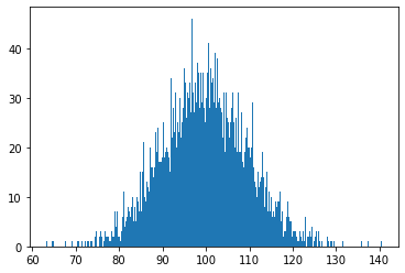
As a human nature, I assume that the abilities of the people are normally distributed. And then I assign the abilities' numbers to the people's ability property.

import numpy as np
import matplotlib.pyplot as plt

# normally distributed abilities
mu = 100
sigma = 10
abilities = np.random.normal(mu, sigma, n)

# assign the abilities to the people
for i in range(n):
    people[i].ability = abilities[i]

The figure below illustrates the distribution of the original abilities of my \(n\) people sample.

# plot the distribution of people's abilities
p_abilities = [p.ability for p in people]
plt.hist(p_abilities, bins=int(n/10))
plt.show()

​

​

Private decisions

In this section, I set several parameters to conduct personal utility maximization. A person can decide the training years on his own condition to maximize his/her present value. And now the \(a_{it}\), the ability after training is equal to his/her wealth.

Several parameters

The parameters including length of life span, discount rates etc should be determined before the analysis.

# assume that the average life-time in the country is 60 years.
l = 60

A person make decision according to the accumulated discounting present value of his/her life. And the formula of the accumulated discounting present value is:

\[V^c_i = a_{ti}\frac{e^{-tr}-e^{-lr}}{r} \]

where \(l\) is the life-span length (the first 10 or 14 years of life is not included in \(l\)) and \(t\) is the training years the determined by the person, \(r\) denotes the discounting rate. The discounting rates for different people is different when they are making decisions. Generally, people with higher ability probably have longer life plan. So, I set a discounting rate negative related to person's original ability in the People class such that:

\[r = r_0-ka_i \]

\(a_{ti}\) denotes the permanent year earning of \(i\) after he received \(t\) years of training, as a result I assume that \(a_{ti}\) could be disputed by such formula:

\[a_{ti} = a_{i}+k a_it+mt \]

It is set that the learning effect is influenced by \(a_i\) and \(t\). I have put the setting of ability after training in the People class.

Decision based on maximization the present value

I restrict the training year choice of people in the t_list, which contains a 20 years choices. The people in my sample can choose the most suitable years to have their training.

# t_list is the optional collection of training years.
t_list = range(21)

import pandas as pd

# Each person choose their own training years.
for person in people:
    ## all possible abilities after training
    possible_a = []
    r = person.r() # discounting rate
    for t in t_list:
        person.training = t
        a_ti = person.ab_t()
        v = a_ti*(np.e**(-t*r)-np.e**(-l*r))/r
        possible_a.append(v)
    ## select the optimal training years
    possible_a_s = pd.Series(possible_a)
    m_t = possible_a_s.argsort()[len(possible_a)-1]
    person.training = m_t

After the circulation above, the property of training of each person in my sample is assigned the optimal training years. And I use the function numpy.argsort() to help them find the biggest present value in their optional collections, which refers my previous article.

o_abilities = []
t_abilities = []
t_selected = []
for person in people:
    o_abilities.append(person.ability)
    t_abilities.append(person.ab_t())
    t_selected.append(person.training)
# people's info
df_info = pd.DataFrame({'Original Ability':o_abilities, 'After-Training Ability':t_abilities, 'Training Years':t_selected})

The information of people with top 10 id numbers in my samples is shown in the table below.

df_info[:10] # top-10 people's info

	Original Ability	After-Training Ability	Training Years
0	101.737300	124.497895	5
1	94.767432	112.139524	4
2	93.792341	111.047422	4
3	103.653573	131.311216	6
4	92.517380	105.343944	3
5	112.496763	151.495987	8
6	105.849145	133.901991	6
7	99.041907	121.398193	5
8	99.495032	121.919286	5
9	90.495949	103.140585	3

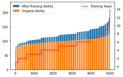
The following chart illustrates the original abilities, abilities after training, and training years selected of each single person in my stochastic sample in a ascending order of the peoples original abilities.

df = df_info.sort_values('Original Ability')
plt.bar(range(n), df['After-Training Ability'], label='After-Training Ability')
plt.bar(range(n), df['Original Ability'], label='Original Ability')
plt.legend()
plt.twinx()
plt.plot(range(n), df['Training Years'], 'red', label='Training Years')
plt.legend(loc=1)
plt.show()

​

​

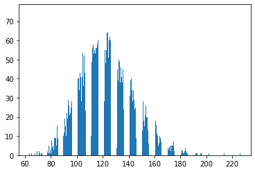
The figure below denotes distribution of the after-training abilities.

# plot the distribution of people's abilities after training
plt.hist(t_abilities, bins=int(n/10))
plt.show()

​

​

Wealth distribution

I test the wealth distribution by skewness. The formula is:

\[SK_1 = \frac{m_3}{m_2^{\frac{3}{2}}}=\frac{\frac{1}{n}\sum_{i=1}^{n}(x_i-\bar x)^3}{(\frac{1}{n}\sum_{i=1}^{n}(x_i-\bar x)^2)^{\frac{3}{2}}} \]

I define two functions to calculate the \(n\)-order moment of the sample and the skewness.

def moment(sample, n):
    sum=0
    for ob in sample:
        sum += ob
    ob_av = sum/len(sample)
    mom = 0
    for ob in sample:
        mom += (1/len(sample))*((ob-ob_av)**n)
    return mom     

def SK1(list):
    sk = moment(list, 3)/((moment(list, 2))**(3/2))
    return sk

Non-training

The skewness of the distribution of original abilities of my sample is calculated below, which is very close to zero.

SK1(o_abilities)

0.012559313586113997

After-training

Compared with the skewness of the distribution of original abilities, the distribution of abilities after training, at the same time, the wealth of the people after human capital investment in my stochastic sample shows a significant positive number, which infers that the distribution depart from symmetry in the direction of positive skewness.

SK1(t_abilities)

0.40574739345316146

A very obvious positive skewness in the group after training, which support my result.