


损失函数总结以及python实现:hinge loss(合页损失)、softmax loss、cross_entropy loss(交叉熵损失)
损失函数在机器学习中的模型非常重要的一部分,它代表了评价模型的好坏程度的标准,最终的优化目标就是通过调整参数去使得损失函数尽可能的小,如果损失函数定义错误或者不符合实际意义的话,训练模型只是在浪费时间。
所以先来了解一下常用的几个损失函数hinge loss(合页损失)、softmax loss、cross_entropy loss(交叉熵损失):
1:hinge loss(合页损失)
又叫Multiclass SVM loss。至于为什么叫合页或者折页函数,可能是因为函数图像的缘故。
s=WX,表示最后一层的输出,维度为(C,None),$L_i$表示每一类的损失,一个样例的损失是所有类的损失的总和。
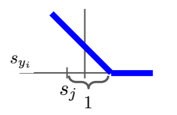
$L_i=\sum_{j!=y_i}\left \{ ^{0 \ \ \ \ \ \ \ \ if \ s_{y_i}\geq s_j+1}_{s_j-s_{y_i}+1 \ otherwise} \right \}$
$ =\sum_{j!=y_i}max(0,s_{y_i}-s_j+1)$
函数图像长这样:
举个例子:
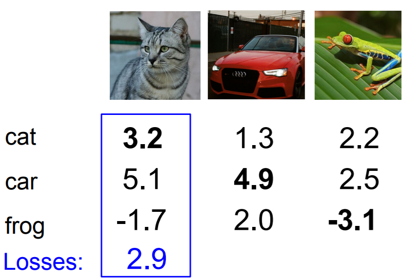
假设我们只有3个类别,上面的图片表示输入,下面3个数字表示最后一层每个类别的分数。
对于第一张猫的图片,$L_i$=max(0, 5.1 - 3.2 + 1) +max(0, -1.7 - 3.2 + 1)=2.9+0=2.9
对于第二张汽车的图片,$L_i$=max(0, 1.3 - 4.9 + 1) +max(0, 2.0 - 4.9 + 1)=0+0=0
可以看到对于分类错误的样例,最后有一个损失产生,对于正确分类的样例,其损失为0.
其实该损失函数不仅仅只是要求正确类别的分数最高,还要高出一定程度。也就是说即使分类正确了也有可能会产生损失,因为有可能正确的类别的分数没有超过错误类别一定的阈值(这里设为1)。但是不管阈值设多少,好像并没有什么太大的意义,只是对应着W的放缩而已。简单的理解就是正确类别的得分不仅要最高,而且要高的比较明显。
对于随机初始化的权重,最终输出应该也不叫均匀,loss应该能得到C-1,可以用这一点来检验自己的损失函数和前向传播的实现是否正确。
2:softmax
softmax操作的意图是把分数转换成概率,来看看怎么转换.
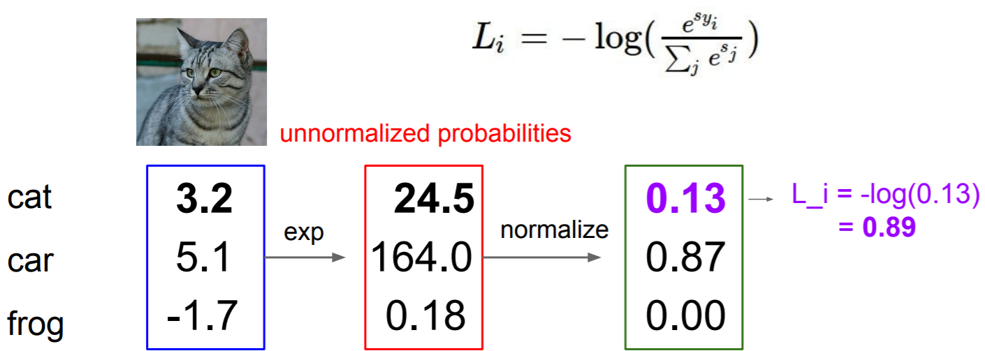
对于输入$x_i$最后会得到C个类别的分数s,每个类别的概率,$P(Y=k|X=x_i)=\frac{e^{s_k}}{\sum_j e^{s_j}}$。
首先取指数次幂,得到整数,然后用比值代替概率。
这样转换了之后我们定义似然函数(也就是损失函数)$L_i=-logP(Y=y_i|X=x_i)$,也就是说正确类别的概率越大越好,这也很好理解。
同样的我们来看一个例子:
同样的,对于随机初始话的权重和数据,$L_i$应该=-log(1/c)。
3:cross_entrop loss
熵的本质是香农信息量的期望。
现有关于样本集的2个概率分布p和q,其中p为真实分布,q非真实分布。按照真实分布p来衡量识别一个样本的所需要的编码长度的期望(即平均编码长度)为:H(p)=-∑p(i)∗logp(i),如果使用错误分布q来表示来自真实分布p的平均编码长度,则应该是:H(p,q)=-∑p(i)∗logq(i)。H(p,q)=-∑p(i)∗logq(i)。因为用q来编码的样本来自分布p,所以期望H(p,q)中概率是p(i)。H(p,q)我们称之为“交叉熵”。
根据公式可以看出,对于正确分类只有一个情况,交叉熵H(p,q)=- ∑logq(i),其中q(i)为正确分类的预测概率,其余的项全部为0,因为除了正确类别,其余的真是概率p(i)都为0.在这种情况下,交叉熵损失与softmax损失其实就是同一回事。
python代码实现:
 1 #首先是线性分类器的类实现 linear_classifier.py
 2
 3 import numpy as np
 4 from linear_svm import *
 5 from softmax import *
 6
 7
 8 class LinearClassifier(object):
 9   #线性分类器的基类
10   def __init__(self):
11     self.W = None
12
13   def train(self, X, y, learning_rate=1e-3, reg=1e-5, num_iters=100,
14             batch_size=200, verbose=False):
15     """
16     使用SGD优化参数矩阵
17
18     Inputs:
19     - X (N, D)
20     - y (N,)
21     - learning_rate: 学习率.
22     - reg: 正则参数.
23     - num_iters: (int) 训练迭代的次数
24     - batch_size: (int) 每次迭代使用的样本数量.
25     - verbose: (boolean) 是否显示训练进度
26
27     Outputs:
28     返回一个list保存了每次迭代的loss
29     """
30     num_train, dim = X.shape
31     num_classes = np.max(y) + 1 # 假设有k类,y的取值为【0,k-1】且最大的下标一定会在训练数据中出现
32
33     #初始化权重矩阵
34     if self.W is None:
35       self.W = 0.001 * np.random.randn(dim, num_classes)
36
37
38     loss_history = []
39     for it in range(num_iters):
40       #在每次迭代,随机选择batch_size个数据
41       mask=np.random.choice(num_train,batch_size,replace=True)
42       X_batch = X[mask]
43       y_batch = y[mask]
44
45       # 计算损失和梯度
46       loss, grad = self.loss(X_batch, y_batch, reg)
47       loss_history.append(loss)
48
49       # 更新参数
50       self.W-=grad*learning_rate
51
52       if verbose and it % 100 == 0:
53         print('iteration %d / %d: loss %f' % (it, num_iters, loss))
54
55     return loss_history
56
57   def predict(self, X):
58     """
59     使用训练好的参数来对输入进行预测
60
61     Inputs:
62     - X (N, D)
63
64     Returns:
65     - y_pred (N,):预测的正确分类的下标
66     """
67
68     y_pred=np.dot(X,self.W)
69     y_pred = np.argmax(y_pred, axis = 1)
70
71     return y_pred
72
73   def loss(self, X_batch, y_batch, reg):
74     """
75     这只是一个线性分类器的基类
76     不同的线性分类器loss的计算方式不同
77     所以需要在子类中重写
78     """
79     pass
80
81
82 class LinearSVM(LinearClassifier):
83   """ 使用SVM loss """
84
85   def loss(self, X_batch, y_batch, reg):
86     return svm_loss_vectorized(self.W, X_batch, y_batch, reg)
87
88
89 class Softmax(LinearClassifier):
90   """ 使用交叉熵 """
91
92   def loss(self, X_batch, y_batch, reg):
93     return softmax_loss_vectorized(self.W, X_batch, y_batch, reg)
 1 #svm loss 的实现 softmax.py
 2
 3 import numpy as np
 4 from random import shuffle
 5
 6 def softmax_loss_naive(W, X, y, reg):
 7   """
 8   用循环实现softmax损失函数
 9   D,C,N分别表示数据维度,标签种类个数和数据批大小
10   Inputs:
11   - W (D, C):weights.
12   - X (N, D):data.
13   - y (N,): labels
14   - reg: (float) regularization strength
15
16   Returns :
17   - loss
18   - gradient
19   """
20
21   loss = 0.0
22   dW = np.zeros_like(W)
23
24   num_classes = W.shape[1]
25   num_train = X.shape[0]
26
27   for i in range(num_train):
28     scores=np.dot(X[i],W)
29     shift_scores=scores-max(scores)
30     dom=np.log(np.sum(np.exp(shift_scores)))
31     loss_i=-shift_scores[y[i]]+dom
32     loss+=loss_i
33     for j in range(num_classes):
34       softmax_output = np.exp(shift_scores[j])/sum(np.exp(shift_scores))
35       if j == y[i]:
36         dW[:,j] += (-1 + softmax_output) *X[i].T
37       else:
38         dW[:,j] += softmax_output *X[i].T
39   loss /= num_train
40   loss += reg * np.sum(W * W)
41   dW = dW/num_train + 2*reg* W
42
43
44   return loss, dW
45
46
47 def softmax_loss_vectorized(W, X, y, reg):
48   """
49   无循环的实现
50   """
51
52   loss = 0.0
53   dW = np.zeros_like(W)
54   num_classes = W.shape[1]
55   num_train = X.shape[0]
56
57   scores=np.dot(X,W)
58   shift_scores=scores-np.max(scores,axis=1).reshape(-1,1)
59   softmax_output = np.exp(shift_scores)/np.sum(np.exp(shift_scores), axis = 1).reshape(-1,1)
60   loss=np.sum(-np.log(softmax_output[range(num_train),y]))
61   loss=loss/num_train+reg * np.sum(W * W)
62
63   dW=softmax_output.copy()
64   dW[range(num_train),y]-=1
65   dW=np.dot(X.T,dW)
66   dW = dW/num_train + 2*reg* W
67
68
69   return loss, dW
 1 #svm loss的实现 linear_svm.py
 2
 3 import numpy as np
 4 from random import shuffle
 5
 6 def svm_loss_naive(W, X, y, reg):
 7   """
 8   用循环实现的SVM loss计算
 9   这里的loss函数使用的是margin loss
10
11   Inputs:
12   - W (D, C): 权重矩阵.
13   - X (N, D): 批输入
14   - y (N,) 标签
15   - reg: 正则参数
16
17   Returns :
18   - loss float
19   - W的梯度
20   """
21   dW = np.zeros(W.shape)
22   num_classes = W.shape[1]
23   num_train = X.shape[0]
24   loss = 0.0
25
26   for i in range(num_train):
27     scores = X[i].dot(W)
28     correct_class_score = scores[y[i]]
29     for j in range(num_classes):
30       if j == y[i]:
31         continue
32       margin = scores[j] - correct_class_score + 1
33       if margin > 0:
34         loss += margin
35         dW[:,j]+=X[i].T
36         dW[:,y[i]]-=X[i].T
37
38
39   loss /= num_train
40   dW/=num_train
41   loss += reg * np.sum(W * W)
42   dW+=2* reg * W
43
44
45   return loss, dW
46
47
48 def svm_loss_vectorized(W, X, y, reg):
49   """
50   不使用循环,利用numpy矩阵运算的特性实现loss和梯度计算
51   """
52   loss = 0.0
53   dW = np.zeros(W.shape)
54
55   #计算loss
56   num_classes = W.shape[1]
57   num_train = X.shape[0]
58   scores=np.dot(X,W)#得到得分矩阵(N,C)
59   correct_socre=scores[range(num_train), list(y)].reshape(-1,1)#得到每个输入的正确分类的分数
60   margins=np.maximum(0,scores-correct_socre+1)
61   margins[range(num_train), list(y)] = 0
62   loss=np.sum(margins)/num_train+reg * np.sum(W * W)
63
64   #计算梯度
65   mask=np.zeros((num_train,num_classes))
66   mask[margins>0]=1
67   mask[range(num_train),list(y)]-=np.sum(mask,axis=1)
68   dW=np.dot(X.T,mask)
69   dW/=num_train
70   dW+=2* reg * W
71
72   return loss, dW
  1 #最后是测试文件,看看实现的线性分类器在CIFAR10上的分类效果如何
  2
  3 # coding: utf-8
  4
  5 #实现hinge_loss和sotfmax_loss
  6
  7 import random
  8 import numpy as np
  9 from cs231n.data_utils import load_CIFAR10
 10 import matplotlib.pyplot as plt
 11 from cs231n.classifiers.linear_svm import svm_loss_naive,svm_loss_vectorized
 12 from cs231n.classifiers.softmax import softmax_loss_naive,softmax_loss_vectorized
 13 import time
 14 from cs231n.classifiers import LinearSVM,Softmax
 15 %matplotlib inline
 16 plt.rcParams['figure.figsize'] = (10.0, 8.0) # set default size of plots
 17 plt.rcParams['image.interpolation'] = 'nearest'
 18 plt.rcParams['image.cmap'] = 'gray'
 19
 20
 21 #######################################################################################
 22 #######################################################################################
 23 ###################################第一部分 载入数据并处理###############################
 24 #######################################################################################
 25 #######################################################################################
 26
 27 # 载入CIFAR10数据.
 28 cifar10_dir = 'cs231n/datasets/cifar-10-batches-py'
 29 X_train, y_train, X_test, y_test = load_CIFAR10(cifar10_dir)
 30
 31 print('Training data shape: ', X_train.shape)
 32 print('Training labels shape: ', y_train.shape)
 33 print('Test data shape: ', X_test.shape)
 34 print('Test labels shape: ', y_test.shape)
 35
 36 #每个分类选几个图片显示观察一下
 37 classes = ['plane', 'car', 'bird', 'cat', 'deer', 'dog', 'frog', 'horse', 'ship', 'truck']
 38 num_classes = len(classes)
 39 samples_per_class = 7
 40 for y, cls in enumerate(classes):
 41     idxs = np.flatnonzero(y_train == y)
 42     idxs = np.random.choice(idxs, samples_per_class, replace=False)
 43     for i, idx in enumerate(idxs):
 44         plt_idx = i * num_classes + y + 1
 45         plt.subplot(samples_per_class, num_classes, plt_idx)
 46         plt.imshow(X_train[idx].astype('uint8'))
 47         plt.axis('off')
 48         if i == 0:
 49             plt.title(cls)
 50 plt.show()
 51
 52 #把数据分为训练集,验证集和测试集。
 53 #用一个小子集做测验,运行更快。
 54 num_training = 49000
 55 num_validation = 1000
 56 num_test = 1000
 57 num_dev = 500
 58
 59 #数据集本身没有给验证集,需要自己把训练集分成两部分
 60 mask = range(num_training, num_training + num_validation)
 61 X_val = X_train[mask]
 62 y_val = y_train[mask]
 63
 64 mask = range(num_training)
 65 X_train = X_train[mask]
 66 y_train = y_train[mask]
 67
 68
 69 mask = np.random.choice(num_training, num_dev, replace=False)
 70 X_dev = X_train[mask]
 71 y_dev = y_train[mask]
 72
 73 mask = range(num_test)
 74 X_test = X_test[mask]
 75 y_test = y_test[mask]
 76
 77 print('Train data shape: ', X_train.shape)
 78 print('Train labels shape: ', y_train.shape)
 79 print('Validation data shape: ', X_val.shape)
 80 print('Validation labels shape: ', y_val.shape)
 81 print('Test data shape: ', X_test.shape)
 82 print('Test labels shape: ', y_test.shape)
 83
 84
 85 X_train = np.reshape(X_train, (X_train.shape[0], -1))
 86 X_val = np.reshape(X_val, (X_val.shape[0], -1))
 87 X_test = np.reshape(X_test, (X_test.shape[0], -1))
 88 X_dev = np.reshape(X_dev, (X_dev.shape[0], -1))
 89
 90 print('Training data shape: ', X_train.shape)
 91 print('Validation data shape: ', X_val.shape)
 92 print('Test data shape: ', X_test.shape)
 93 print('dev data shape: ', X_dev.shape)
 94
 95
 96 # 预处理: 把像素点数据化成以0为中心
 97 # 第一步: 在训练集上计算图片像素点的平均值
 98 mean_image = np.mean(X_train, axis=0)
 99 print(mean_image.shape)
100 plt.figure(figsize=(4,4))
101 plt.imshow(mean_image.reshape((32,32,3)).astype('uint8')) # 可视化一下平均值
102 plt.show()
103
104 # 第二步: 所有数据都减去刚刚得到的均值
105 X_train -= mean_image
106 X_val -= mean_image
107 X_test -= mean_image
108 X_dev -= mean_image
109
110
111 # 第三步: 给所有的图片都加一个位,并设为1,这样在训练权重的时候就不需要b了,只需要w
112 # 相当于把b的训练并入了W中
113 X_train = np.hstack([X_train, np.ones((X_train.shape[0], 1))])
114 X_val = np.hstack([X_val, np.ones((X_val.shape[0], 1))])
115 X_test = np.hstack([X_test, np.ones((X_test.shape[0], 1))])
116 X_dev = np.hstack([X_dev, np.ones((X_dev.shape[0], 1))])
117
118 print(X_train.shape, X_val.shape, X_test.shape, X_dev.shape)
119
120
121 #######################################################################################
122 #######################################################################################
123 ###################################第二部分 定义需要用到的函数###########################
124 #######################################################################################
125 #######################################################################################
126
127 def cmp_naiveANDvectorized(naive,vectorized):
128     '''
129     每个损失函数都用两种方式实现:循环和无循环(即利用numpy的特性)
130     '''
131
132     W = np.random.randn(3073, 10) * 0.0001
133
134     #对比两张实现方式的计算时间
135     tic = time.time()
136     loss_naive, grad_naive = naive(W, X_dev, y_dev, 0.000005)
137     toc = time.time()
138     print('Naive computed in %fs' % ( toc - tic))
139
140     tic = time.time()
141     loss_vectorized, grad_vectorized = vectorized(W, X_dev, y_dev, 0.000005)
142     toc = time.time()
143     print('Vectorized  computed in %fs' % ( toc - tic))
144
145     # 检验损失的实现是否正确,对于随机初始化的数据的权重,
146     # softmax_loss应该约等于-log(0.1),svm_loss应该约等于9
147     print('loss %f %f' % (loss_naive , loss_vectorized))
148
149     # 对比两种实现方式得到的结果是否相同
150     print('difference loss %f ' % (loss_naive - loss_vectorized))
151     difference = np.linalg.norm(grad_naive - grad_vectorized, ord='fro')
152     print('difference gradient: %f' % difference)
153
154 def cross_choose(Linear_classifier,learning_rates,regularization_strengths):
155     '''
156     选择超参数
157     '''
158
159     results = {}    # 存储每一对超参数对应的训练集和验证集上的正确率
160     best_val = -1   # 最好的验证集上的正确率
161     best_model = None # 最好的验证集正确率对应的svm类的对象
162     best_loss_hist=None
163     for rs in regularization_strengths:
164         for lr in learning_rates:
165             classifier = Linear_classifier
166             loss_hist = classifier.train(X_train, y_train, lr, rs, num_iters=3000)
167             y_train_pred = classifier.predict(X_train)
168             train_accuracy = np.mean(y_train == y_train_pred)
169             y_val_pred = classifier.predict(X_val)
170             val_accuracy = np.mean(y_val == y_val_pred)
171             if val_accuracy > best_val:
172                 best_val = val_accuracy
173                 best_model = classifier
174                 best_loss_hist=loss_hist
175             results[(lr,rs)] = train_accuracy, val_accuracy
176
177     for lr, reg in sorted(results):
178         train_accuracy, val_accuracy = results[(lr, reg)]
179         print ('lr %e reg %e train accuracy: %f val accuracy: %f' % (
180                     lr, reg, train_accuracy, val_accuracy))
181
182     print('best validation accuracy achieved during cross-validation: %f' % best_val)
183     # 可视化loss曲线
184     plt.plot(best_loss_hist)
185     plt.xlabel('Iteration number')
186     plt.ylabel('Loss value')
187     plt.show()
188     return results,best_val,best_model
189
190 def show_weight(best_model):
191     # 看看最好的模型的效果
192     # 可视化学到的权重
193
194     y_test_pred = best_model.predict(X_test)
195     test_accuracy = np.mean(y_test == y_test_pred)
196     print('final test set accuracy: %f' % test_accuracy)
197
198     w = best_model.W[:-1,:] # 去掉偏置参数
199     w = w.reshape(32, 32, 3, 10)
200     w_min, w_max = np.min(w), np.max(w)
201     classes = ['plane', 'car', 'bird', 'cat', 'deer', 'dog', 'frog', 'horse', 'ship', 'truck']
202     for i in range(10):
203         plt.subplot(2, 5, i + 1)
204
205         # 把权重转换到0-255
206         wimg = 255.0 * (w[:, :, :, i].squeeze() - w_min) / (w_max - w_min)
207         plt.imshow(wimg.astype('uint8'))
208         plt.axis('off')
209         plt.title(classes[i])
210     plt.show()
211
212 #######################################################################################
213 #######################################################################################
214 ##########################第三部分 应用和比较svm_loss和softmax_loss######################
215 #######################################################################################
216 #######################################################################################
217
218 cmp_naiveANDvectorized(svm_loss_naive,svm_loss_vectorized)
219 learning_rates = [(1+i*0.1)*1e-7 for i in range(-3,5)]
220 regularization_strengths = [(5+i*0.1)*1e3 for i in range(-3,3)]
221 #正则参数的选择要根据正常损失和W*W的大小的数量级来确定,初始时正常loss大概是9,W*W大概是1e-6
222 #可以观察最后loss的值的大小来继续调整正则参数的大小,使正常损失和正则损失保持合适的比例
223 results,best_val,best_model=cross_choose(LinearSVM(),learning_rates,regularization_strengths)
224 show_weight(best_model)
225
226 print("--------------------------------------------------------")
227
228 cmp_naiveANDvectorized(softmax_loss_naive,softmax_loss_vectorized)
229 learning_rates = [(2+i*0.1)*1e-7 for i in range(-2,2)]
230 regularization_strengths = [(7+i*0.1)*1e3 for i in range(-3,3)]
231 results,best_val,best_model=cross_choose(Softmax(),learning_rates,regularization_strengths)
232 show_weight(best_model)
 1 #获取数据的部分
 2
 3 from six.moves import cPickle as pickle
 4 import numpy as np
 5 import os
 6 from scipy.misc import imread
 7 import platform
 8
 9 def load_pickle(f):
10     version = platform.python_version_tuple()
11     if version[0] == '2':
12         return  pickle.load(f)
13     elif version[0] == '3':
14         return  pickle.load(f, encoding='latin1')
15     raise ValueError("invalid python version: {}".format(version))
16
17 def load_CIFAR_batch(filename):
18   """ CIRAR的数据是分批的,这个函数的功能是载入一批数据 """
19   with open(filename, 'rb') as f:
20     datadict = load_pickle(f) #以二进制方式打开文件
21     X = datadict['data']
22     Y = datadict['labels']
23     X = X.reshape(10000, 3, 32, 32).transpose(0,2,3,1).astype("float")
24     Y = np.array(Y)
25     return X, Y
26
27 def load_CIFAR10(ROOT):
28   """ load 所有的数据 """
29   xs = []
30   ys = []
31   for b in range(1,6):
32     f = os.path.join(ROOT, 'data_batch_%d' % (b, ))
33     X, Y = load_CIFAR_batch(f)
34     xs.append(X)
35     ys.append(Y)
36   Xtr = np.concatenate(xs)
37   Ytr = np.concatenate(ys)
38   del X, Y
39   Xte, Yte = load_CIFAR_batch(os.path.join(ROOT, 'test_batch'))
40   return Xtr, Ytr, Xte, Yte
41
42
43 def get_CIFAR10_data(num_training=49000, num_validation=1000, num_test=1000,
44                      subtract_mean=True):
45     """
46     Load the CIFAR-10 dataset from disk and perform preprocessing to prepare
47     it for classifiers. These are the same steps as we used for the SVM, but
48     condensed to a single function.
49     """
50     # Load the raw CIFAR-10 data
51     cifar10_dir = 'cs231n/datasets/cifar-10-batches-py'
52     X_train, y_train, X_test, y_test = load_CIFAR10(cifar10_dir)
53
54     # Subsample the data
55     mask = list(range(num_training, num_training + num_validation))
56     X_val = X_train[mask]
57     y_val = y_train[mask]
58     mask = list(range(num_training))
59     X_train = X_train[mask]
60     y_train = y_train[mask]
61     mask = list(range(num_test))
62     X_test = X_test[mask]
63     y_test = y_test[mask]
64
65     # Normalize the data: subtract the mean image
66     if subtract_mean:
67       mean_image = np.mean(X_train, axis=0)
68       X_train -= mean_image
69       X_val -= mean_image
70       X_test -= mean_image
71
72     # Transpose so that channels come first
73     X_train = X_train.transpose(0, 3, 1, 2).copy()
74     X_val = X_val.transpose(0, 3, 1, 2).copy()
75     X_test = X_test.transpose(0, 3, 1, 2).copy()
76
77     # Package data into a dictionary
78     return {
79       'X_train': X_train, 'y_train': y_train,
80       'X_val': X_val, 'y_val': y_val,
81       'X_test': X_test, 'y_test': y_test,
82     }

 浙公网安备 33010602011771号