NumPy学习笔记：2、NumPy数组运算

一、元素级运算（注意：进行运算的两个数组必须有相同的shape，否则会报错）

1、标量运算

>>> a = np.array([1, 2, 3, 4])
>>> a + 1
array([2, 3, 4, 5])
>>> 2**a
array([ 2,  4,  8, 16])

2、与另一个数组的数学运算

>>> b = np.ones(4) + 1
>>> a - b
array([-1.,  0.,  1.,  2.])
>>> a * b   # ！！！并非矩阵乘法，只是单纯的对应元素相乘
array([ 2.,  4.,  6.,  8.])

>>> j = np.arange(5)
>>> 2**(j + 1) - j
array([ 2,  3,  6, 13, 28])

注意，矩阵的乘法运算如下：

>>> c = np.ones((3,3))
>>> c
array([[ 1.,  1.,  1.],
       [ 1.,  1.,  1.],
       [ 1.,  1.,  1.]])
>>> c.dot(c)    # 矩阵乘法
array([[ 3.,  3.,  3.],
       [ 3.,  3.,  3.],
       [ 3.,  3.,  3.]])

3、比较运算（比较的是两个数组中的每一个元素）

>>> a = np.array([1, 2, 3, 4])
>>> b = np.array([4, 2, 2, 4])
>>> a == b
array([False,  True, False,  True], dtype=bool)
>>> a > b
array([False, False,  True, False], dtype=bool)

注意，比较两个数组是否相同：

>>> a = np.array([1,2,3,4])
>>> b = np.array([4,3,2,1])
>>> c = np.array([1,2,3,4])
>>> np.array_equal(a,b)
False
>>> np.array_equal(a,c)
True

4、逻辑运算

>>> a = np.array([1, 1, 0, 0], dtype=bool)
>>> b = np.array([1, 0, 1, 0], dtype=bool)
>>> np.logical_or(a, b)  # 逻辑或
array([ True,  True,  True, False], dtype=bool)
>>> np.logical_and(a, b)  # 逻辑且
array([ True, False, False, False], dtype=bool)

5、超越函数运算

>>> a = np.arange(5)
>>> np.sin(a)   # 正弦
array([ 0.        ,  0.84147098,  0.90929743,  0.14112001, -0.7568025 ])
>>> np.log(a)  # 以自然常数e为底的对数函数
array([       -inf,  0.        ,  0.69314718,  1.09861229,  1.38629436])
>>> np.exp(a)  #以自然常数e为底的指数函数
array([  1.        ,   2.71828183,   7.3890561 ,  20.08553692,  54.59815003])

6、转置（注意，转置运算得到的是一个视图，所以无法进行 a += a.T 运算）

>>> a = np.triu(np.ones((3, 3)), 1)   # see help(np.triu)
>>> a
array([[ 0.,  1.,  1.],
       [ 0.,  0.,  1.],
       [ 0.,  0.,  0.]])
>>> a.T
array([[ 0.,  0.,  0.],
       [ 1.,  0.,  0.],
       [ 1.,  1.,  0.]])

二、降维运算

1、求和

>>> x = np.array([1, 2, 3, 4])
>>> np.sum(x)
10
>>> x.sum()
10

# 计算数组某个维度的和
>>> x = np.array([[1, 1], [2, 2]])
>>> x
array([[1, 1],
       [2, 2]])
>>> x.sum(axis=0)   # 列（第一个维度）
array([3, 3])
>>> x[:, 0].sum(), x[:, 1].sum()
(3, 3)
>>> x.sum(axis=1)   # 行 (第二个维度)
array([2, 4])
>>> x[0, :].sum(), x[1, :].sum()
(2, 4)

2、求极值

>>> x = np.array([1, 3, 2])
>>> x.min()
1
>>> x.max()
3

>>> x.argmin()  # 极小值的最小下标
0
>>> x.argmax()  # 极大值的最小下标
1

3、逻辑运算（注意，括号中的参数为布尔型列表或数组）

>>> np.all([True, True, False])
False
>>> np.any([True, True, False])
True

# 也可以用于数组的比较
>>> a = np.zeros((100, 100))
>>> np.any(a != 0)
False
>>> np.all(a == a)
True

>>> a = np.array([1, 2, 3, 2])
>>> b = np.array([2, 2, 3, 2])
>>> c = np.array([6, 4, 4, 5])
>>> ((a <= b) & (b <= c)).all()
True

4、一些统计值的计算

>>> x = np.array([1, 2, 3, 1])
>>> y = np.array([[1, 2, 3], [5, 6, 1]])
>>> x.mean()  # 平均数
1.75
>>> np.median(x)  # 中位数
1.5
>>> np.median(y, axis=-1) # 每一行的中位数
array([ 2.,  5.])

>>> x.std()          # 总体标准差
0.82915619758884995

三、广播

 Numpy数组的基本运算操作都是元素级的，进行运算的两个数组需要具有相同的大小。

然而，如果Numpy可以把不同大小的数组转换成相同大小的数组，他们就可以进行运算了。这种转换成为广播。

这种转换如下图所示：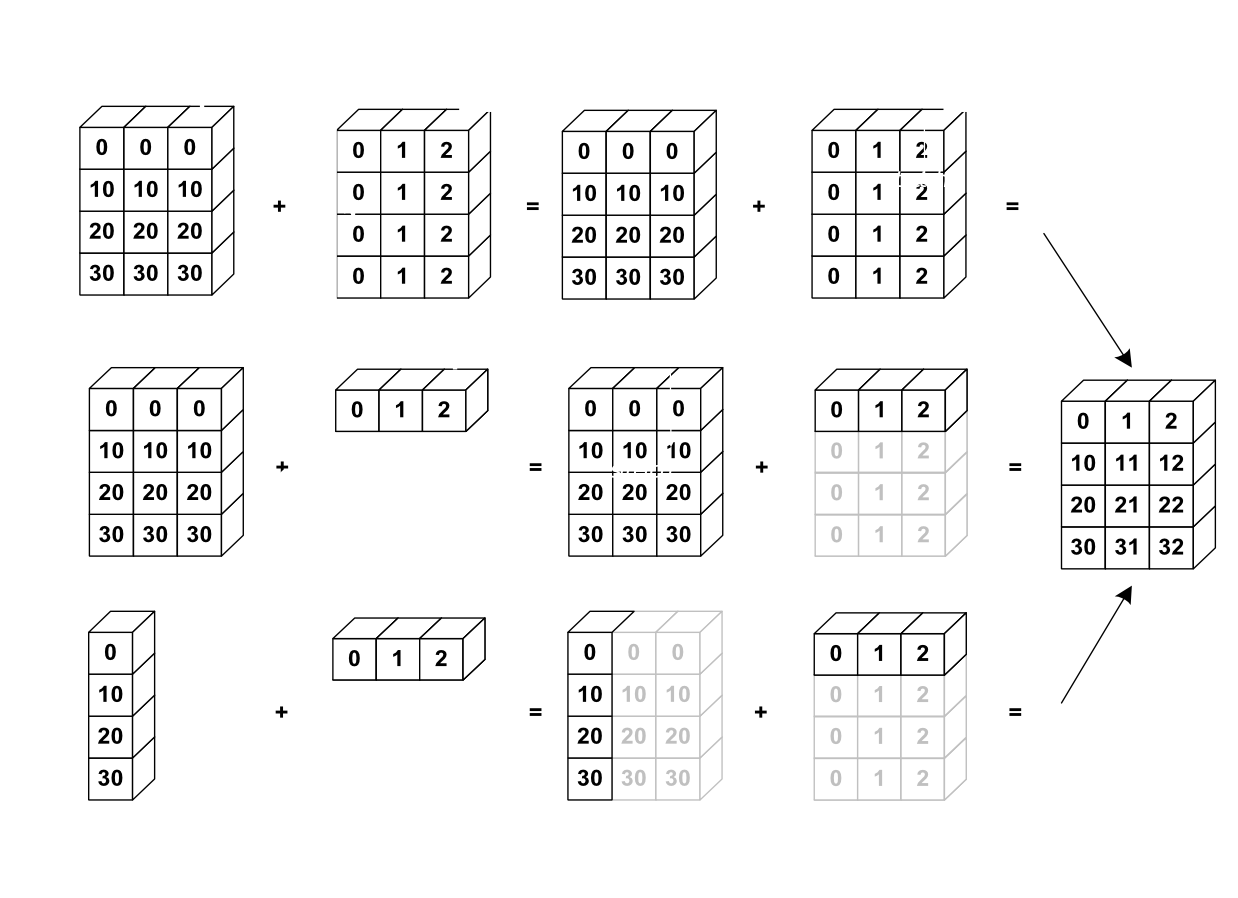

>>> a = np.tile(np.arange(0, 40, 10), (3, 1)).T
>>> a
array([[ 0,  0,  0],
       [10, 10, 10],
       [20, 20, 20],
       [30, 30, 30]])
>>> b = np.array([0, 1, 2])
>>> a + b
array([[ 0,  1,  2],
       [10, 11, 12],
       [20, 21, 22],
       [30, 31, 32]])

>>> a = np.arange(0, 40, 10)
>>> a.shape
(4,)
>>> a = a[:, np.newaxis]  # adds a new axis -> 2D array
>>> a.shape
(4, 1)
>>> a
array([[ 0],
       [10],
       [20],
       [30]])
>>> a + b
array([[ 0,  1,  2],
       [10, 11, 12],
       [20, 21, 22],
       [30, 31, 32]])

注意： np.ogrid() 和 np.mgrid() 的应用。

四、Numpy数组的形状的操作

1、Flatting

>>> a = np.array([[1, 2, 3], [4, 5, 6]])
>>> a.ravel()
array([1, 2, 3, 4, 5, 6])
>>> a.T
array([[1, 4],
       [2, 5],
       [3, 6]])
>>> a.T.ravel()
array([1, 4, 2, 5, 3, 6])

对于更高维数组，最末的维度最先ravel。

注意：flatten 和 ravel 的区别，哪一个创建的是视图，哪一个创建的是副本。

2、Reshaping（与Flatting操作正好相反）

>>> a.shape
(2, 3)
>>> b = a.ravel()
>>> b = b.reshape((2, 3))
>>> b
array([[1, 2, 3],
       [4, 5, 6]])
>>> a.reshape((2, -1))    # unspecified (-1) value is inferred
array([[1, 2, 3],
       [4, 5, 6]])

 

ndarray.reshape() 可能会返回一个视图，也可能返回一个副本。需看具体情况确认。

3、Adding a dimension - 增加一个维度

带有 np.newaxis 的索引的数组对象可以为这个数组对象增加一个维度。

>>> z = np.array([1, 2, 3])
>>> z
array([1, 2, 3])

>>> z[:, np.newaxis]
array([[1],
       [2],
       [3]])

>>> z[np.newaxis, :]
array([[1, 2, 3]])

4、Dimension shuffling - 维度转化

>>> a = np.arange(4*3*2).reshape(4, 3, 2)
>>> a.shape
(4, 3, 2)
>>> a[0, 2, 1]
5
>>> b = a.transpose(1, 2, 0)
>>> b.shape
(3, 2, 4)
>>> b[2, 1, 0]
5

ndarray.transpose 创建的是一个视图。

5、Resizing - 重新定义大小

>>> a = np.arange(4)
>>> a.resize((8,))
>>> a
array([0, 1, 2, 3, 0, 0, 0, 0])

注意：一个数组必须没有其他指向它的对象，它的大小才能被重新定义。

五、数据的排序

1、依据某一个维度进行排序（原数组不变）

>>> a = np.array([[4, 3, 5], [1, 2, 1]])
>>> b = np.sort(a, axis=1)   # 单独对行进行排序
>>> b
array([[3, 4, 5],
       [1, 1, 2]])

2、数组本身进行排序（原数组变为排序后的数组）

>>> a.sort(axis=1)
>>> a
array([[3, 4, 5],
       [1, 1, 2]])

3、查找最小值和最大值

>>> a = np.array([4, 3, 1, 2])
>>> j_max = np.argmax(a)
>>> j_min = np.argmin(a)
>>> j_max, j_min
(0, 2)

六、总结

What do you need to know to get started?

• Know how to create arrays : array, arange, ones, zeros.

• Know the shape of the array with array.shape, then use slicing to obtain different views of the array: array[::2], etc. Adjust the shape of the array using reshape or flatten it with ravel.

• Obtain a subset of the elements of an array and/or modify their values with masks

• Know miscellaneous operations on arrays, such as finding the mean or max (array.max(), array.mean()). No need to retain everything, but have the reflex to search in the documentation (online docs, help(), lookfor())!!

• For advanced use: master the indexing with arrays of integers, as well as broadcasting. Know more NumPy functions to handle various array operations.