机器学习-线性回归和多项式回归

 线性回归模型

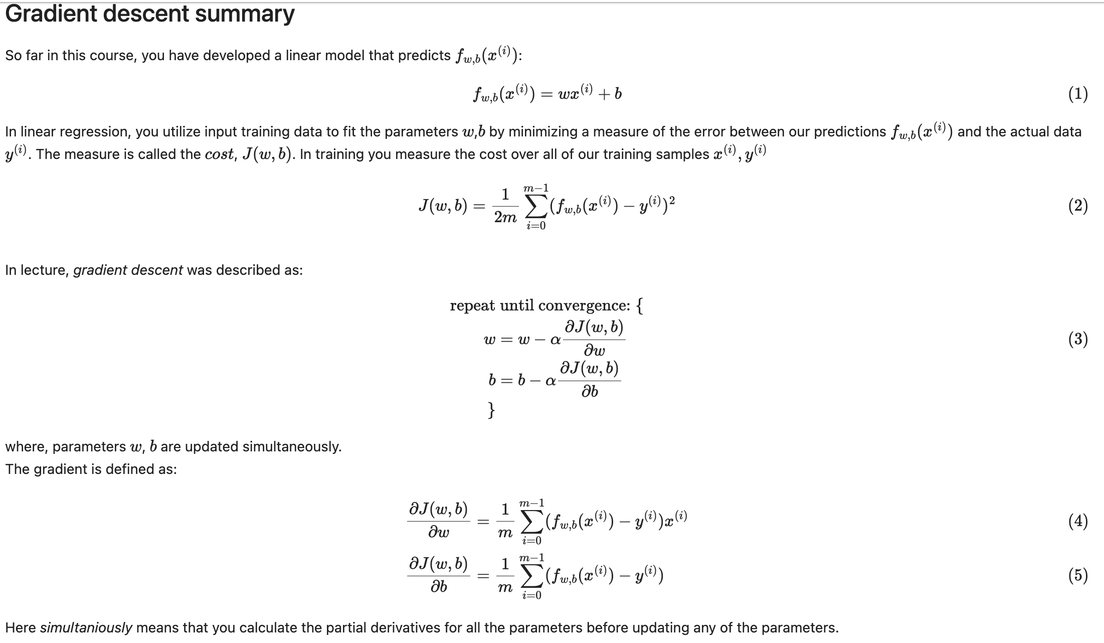
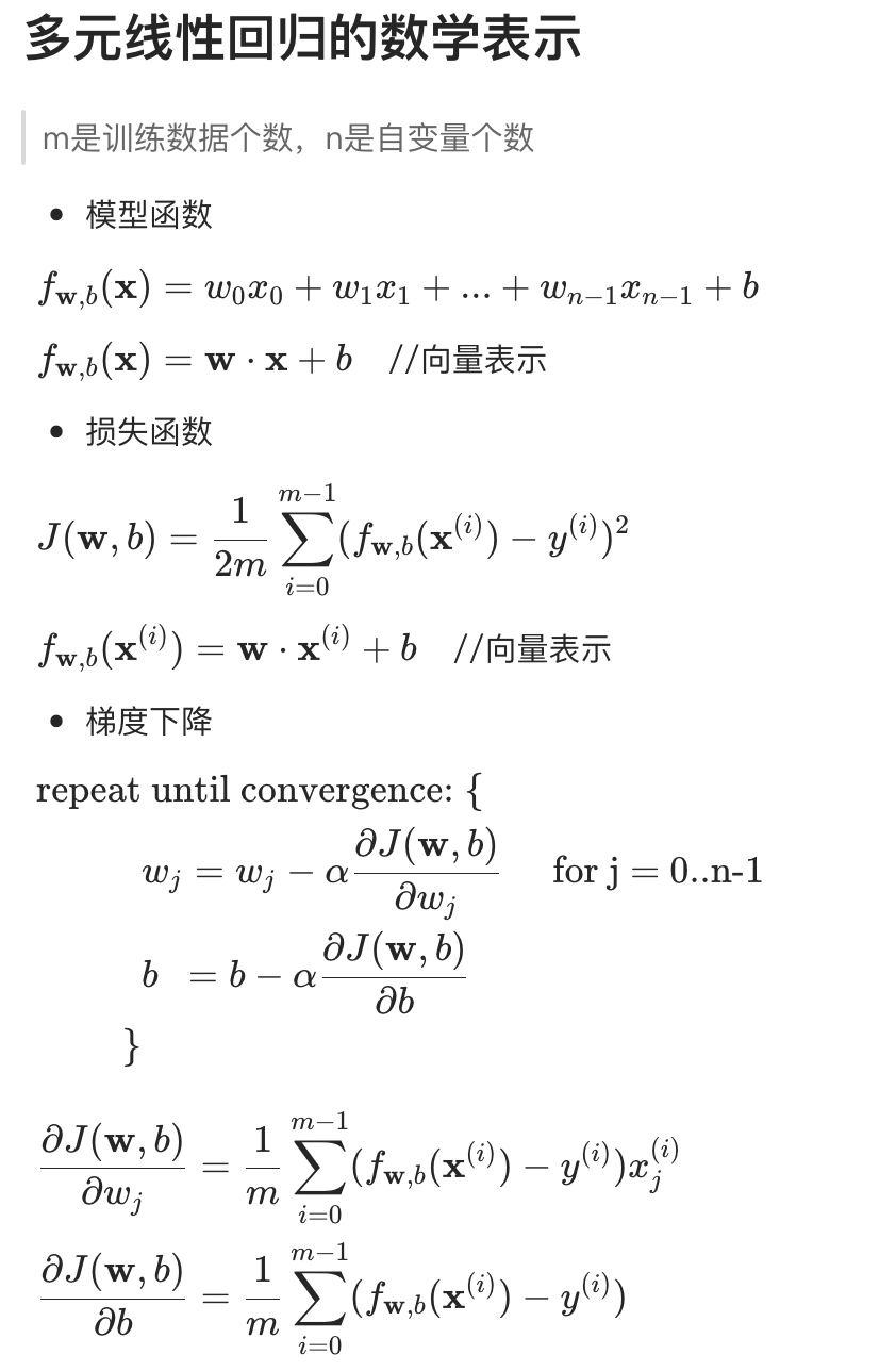
多元线性回归模型

 

多元线性回归模型实例

源数据

The housing data was derived from the Ames Housing dataset compiled by Dean De Cock for use in data science education. 

代码实现

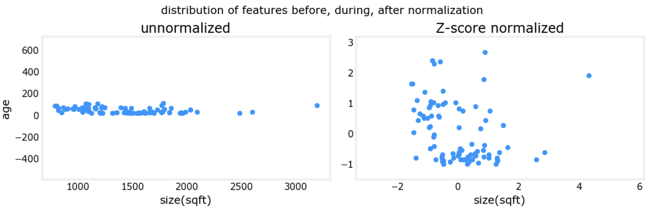
z-score标准化

# z-score标准化
def zscore_normalize_features(X):
    mu = np.mean(X, axis=0)  # MUST SET  axis=0
    sigma = np.std(X, axis=0)  # MUST SET  axis=0
    x_norm = (X - mu)/sigma
    return x_norms

损失函数

def compute_cost(x_train, y, w, b):
    '''
    m : 训练数据个数
    n : 自变量个数
    '''
    m = x_train.shape[0]
    sum_cost = 0
    for idx in range(m):
        f_wb = np.dot(x_train[idx], w) + b
        cost = (f_wb - y[idx])**2
        sum_cost += cost
    sum_cost = sum_cost/(2*m)
    return sum_cost

计算梯度

def compute_gradient(x_train, y, w, b):
    '''
    m : 训练数据个数
    n : 自变量个数
    '''
    m, n = x_train.shape
    sum_w = np.zeros(n)
    sum_b = 0
    for idx in range(m):
        f_wb = np.dot(x_train[idx], w) + b
        diff = f_wb - y[idx]
        sum_w += diff * x_train[idx]
        sum_b += diff
    w_gradient = sum_w / m
    b_gradient = sum_b / m
    return w_gradient, b_gradient

梯度下降实现

def gradient_descent(x_train, y, iter_cnt, alpha, func_cost, func_gradient):
    m, n = x_train.shape
    w_initial = np.zeros(n)
    b_initial = 0
    cost_list = []
    w_history = []
    b_history = []
    cnt = int(iter_cnt / 10)
    for idx in range(iter_cnt):
        w_g, b_g = func_gradient(x_train, y, w_initial, b_initial)
        w_initial = w_initial - alpha * w_g
        b_initial = b_initial - alpha * b_g
        w_history.append(w_initial)
        b_history.append(b_initial)
        # 先计算梯度，再计算损失
        _c = func_cost(x_train, y, w_initial, b_initial)
        cost_list.append(_c)
        if idx == 0:
            print(f"[第{idx+1}次] cost: {_c:e}, w: {w_initial}, b: {b_initial:e}")
        if (idx+1) % cnt == 0:
            print(f"[第{idx+1}次] cost: {_c:e}, w: {w_initial}, b: {b_initial:e}")
    return cost_list, w_history, b_history, w_initial, b_initial

main()

import numpy as np
np.set_printoptions(precision=2)
import matplotlib.pyplot as plt


# 数据载入
data = np.loadtxt("./data/houses.txt", delimiter=',', skiprows=1)
X_train = data[:,:4]
y_train = data[:,4]

# 数据标准化
X_norm = zscore_normalize_features_fixed(X_train)
fig,ax=plt.subplots(1, 2, figsize=(12, 4))
ax[0].scatter(X_train[:,0], X_train[:,3])
ax[0].set_xlabel(X_features[0]); ax[0].set_ylabel(X_features[3]);
ax[0].set_title("unnormalized")
ax[0].axis('equal')
ax[1].scatter(X_norm[:,0], X_norm[:,3])
ax[1].set_xlabel(X_features[0]); ax[0].set_ylabel(X_features[3]);
ax[1].set_title(r"Z-score normalized")
ax[1].axis('equal')
plt.tight_layout(rect=[0, 0.03, 1, 0.95])
fig.suptitle("distribution of features before, during, after normalization")
plt.show()

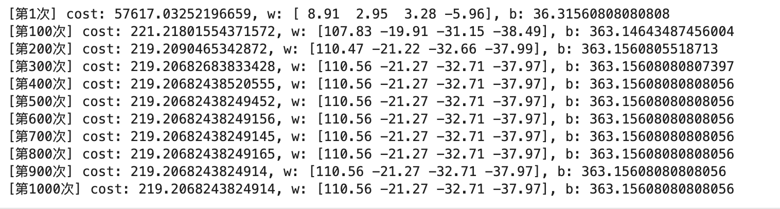
# 开始训练
alpha = 1.0e-1
cost_list_norm, w_history_norm, b_history_norm, w_final_norm, b_final_norm = gradient_descent(X_norm, y_train, 1000, alpha, compute_cost, compute_gradient)
# 检验训练结果
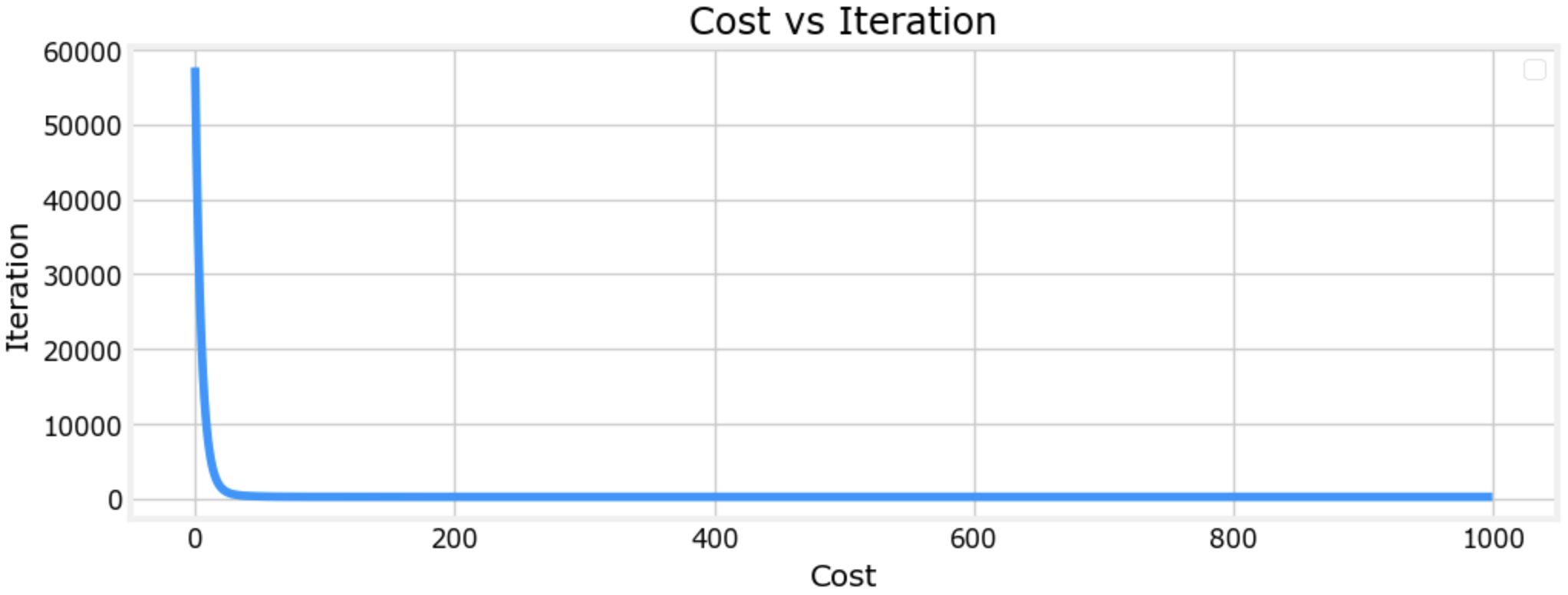
plt.figure(figsize=(12, 4))
plt.plot(cost_list_norm)
plt.title("Cost vs Iteration")
plt.xlabel('Cost')
plt.ylabel('Iteration')
plt.legend()
plt.grid()
plt.show()

执行结果

 

 

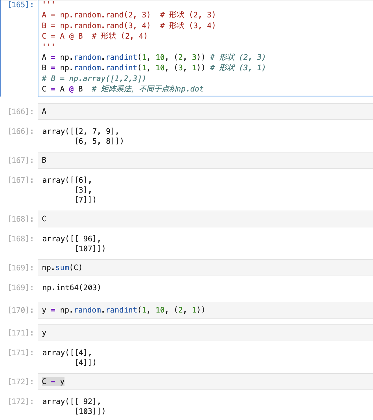
矩阵乘法版本

矩阵乘法示例

代码实现

# Loop version of multi-variable compute_cost
def compute_cost(X, y, w, b): 
    """
    compute cost
    Args:
      X : (ndarray): Shape (m,n) matrix of examples with multiple features
      w : (ndarray): Shape (n)   parameters for prediction   
      b : (scalar):              parameter  for prediction   
    Returns
      cost: (scalar)             cost
    """
    m = X.shape[0]
    cost = 0.0
    for i in range(m):                                
        f_wb_i = np.dot(X[i],w) + b       
        cost = cost + (f_wb_i - y[i])**2              
    cost = cost/(2*m)                                 
    return(np.squeeze(cost)) 


# Matrix version of multi-variable compute_cost
def compute_cost_matrix(X, y, w, b, verbose=False):
    """
    Computes the gradient for linear regression 
     Args:
      X : (array_like Shape (m,n)) variable such as house size 
      y : (array_like Shape (m,)) actual value 
      w : (array_like Shape (n,)) parameters of the model 
      b : (scalar               ) parameter of the model 
      verbose : (Boolean) If true, print out intermediate value f_wb
    Returns
      cost: (scalar)                      
    """ 
    m,n = X.shape

    # calculate f_wb for all examples.
    f_wb = X @ w + b  
    # calculate cost
    total_cost = (1/(2*m)) * np.sum((f_wb-y)**2)

    if verbose: print("f_wb:")
    if verbose: print(f_wb)
        
    return total_cost


# Matrix version of multi-variable compute_gradient
def compute_gradient(X, y, w, b): 
    """
    Computes the gradient for linear regression 
    Args:
      X : (ndarray Shape (m,n)) matrix of examples 
      y : (ndarray Shape (m,))  target value of each example
      w : (ndarray Shape (n,))  parameters of the model      
      b : (scalar)              parameter of the model      
    Returns
      dj_dw : (ndarray Shape (n,)) The gradient of the cost w.r.t. the parameters w. 
      dj_db : (scalar)             The gradient of the cost w.r.t. the parameter b. 
    """
    m,n = X.shape           #(number of examples, number of features)
    dj_dw = np.zeros((n,))
    dj_db = 0.

    for i in range(m):                             
        err = (np.dot(X[i], w) + b) - y[i]   
        for j in range(n):                         
            dj_dw[j] = dj_dw[j] + err * X[i,j]    
        dj_db = dj_db + err                        
    dj_dw = dj_dw/m                                
    dj_db = dj_db/m                                
        
    return dj_db,dj_dw


# Matrix version of multi-variable compute_gradient
def compute_gradient_matrix(X, y, w, b): 
    """
    Computes the gradient for linear regression 
 
    Args:
      X : (array_like Shape (m,n)) variable such as house size 
      y : (array_like Shape (m,1)) actual value 
      w : (array_like Shape (n,1)) Values of parameters of the model      
      b : (scalar )                Values of parameter of the model      
    Returns
      dj_dw: (array_like Shape (n,1)) The gradient of the cost w.r.t. the parameters w. 
      dj_db: (scalar)                The gradient of the cost w.r.t. the parameter b. 
                                  
    """
    m,n = X.shape
    f_wb = X @ w + b              
    e   = f_wb - y                
    dj_dw  = (1/m) * (X.T @ e)    
    dj_db  = (1/m) * np.sum(e)    
        
    return dj_db,dj_dw


def gradient_descent(X, y, w_in, b_in, cost_function, gradient_function, alpha, num_iters): 
    """
    Performs batch gradient descent to learn theta. Updates theta by taking 
    num_iters gradient steps with learning rate alpha
    
    Args:
      X : (array_like Shape (m,n)    matrix of examples 
      y : (array_like Shape (m,))    target value of each example
      w_in : (array_like Shape (n,)) Initial values of parameters of the model
      b_in : (scalar)                Initial value of parameter of the model
      cost_function: function to compute cost
      gradient_function: function to compute the gradient
      alpha : (float) Learning rate
      num_iters : (int) number of iterations to run gradient descent
    Returns
      w : (array_like Shape (n,)) Updated values of parameters of the model after
          running gradient descent
      b : (scalar)                Updated value of parameter of the model after
          running gradient descent
    """
    
    # number of training examples
    m = len(X)
    
    # An array to store values at each iteration primarily for graphing later
    hist={}
    hist["cost"] = []; hist["params"] = []; hist["grads"]=[]; hist["iter"]=[];
    
    w = copy.deepcopy(w_in)  #avoid modifying global w within function
    b = b_in
    save_interval = np.ceil(num_iters/10000) # prevent resource exhaustion for long runs

    for i in range(num_iters):

        # Calculate the gradient and update the parameters
        dj_db,dj_dw = gradient_function(X, y, w, b)   

        # Update Parameters using w, b, alpha and gradient
        w = w - alpha * dj_dw               
        b = b - alpha * dj_db               
      
        # Save cost J,w,b at each save interval for graphing
        if i == 0 or i % save_interval == 0:     
            hist["cost"].append(cost_function(X, y, w, b))
            hist["params"].append([w,b])
            hist["grads"].append([dj_dw,dj_db])
            hist["iter"].append(i)

        # Print cost every at intervals 10 times or as many iterations if < 10
        if i% math.ceil(num_iters/10) == 0:
            print(f"Iteration {i:4d}: Cost {cost_function(X, y, w, b):8.2f}   ")
            cst = cost_function(X, y, w, b)
            print(f"Iteration {i:9d}, Cost: {cst:0.5e}")
    return w, b, hist #return w,b and history for graphing


def run_gradient_descent(X,y,iterations=1000, alpha = 1e-6):
    m,n = X.shape
    # initialize parameters
    initial_w = np.zeros(n)
    initial_b = 0
    # run gradient descent
    w_out, b_out, hist_out = gradient_descent(X ,y, initial_w, initial_b, compute_cost, compute_gradient_matrix, alpha, iterations)
    print(f"w,b found by gradient descent: w: {w_out}, b: {b_out:0.4f}")
    return(w_out, b_out)

多项式回归

x = np.arange(0,20,1)
y = np.cos(x/2)

# f_wb(x) = w0*x + w1*x**2 + w2*x**3 + w3*x**4 + w4*x**5
X = np.c_[x, x**2, x**3, x**4, x**5]
X = zscore_normalize_features(X)
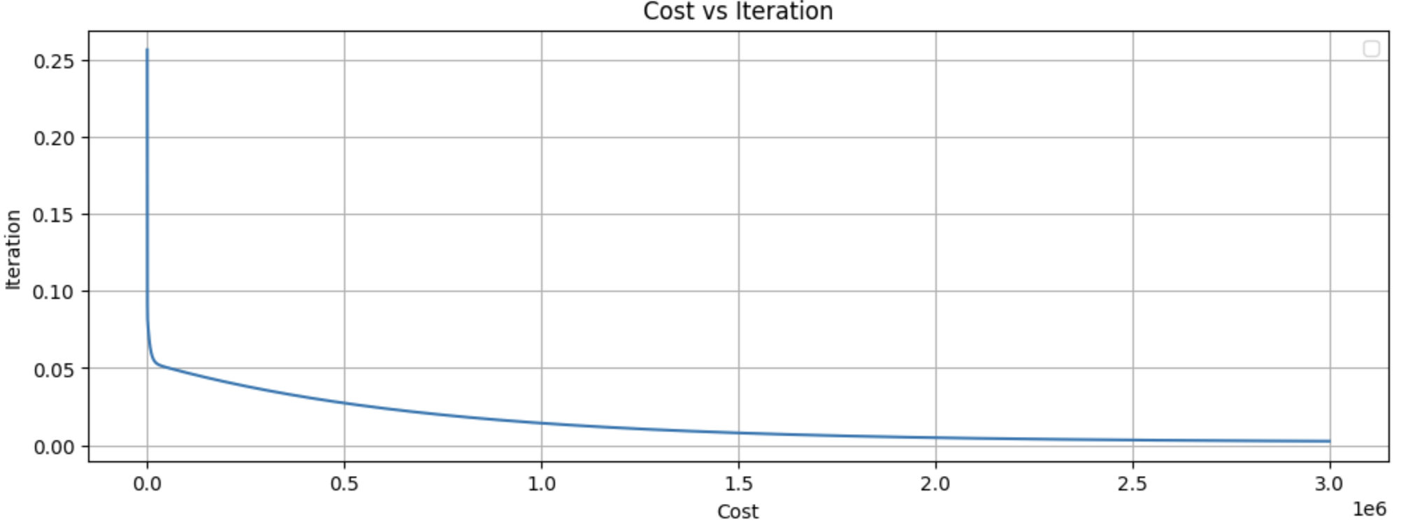
cost_list, w_history, b_history, w_final, b_final = gradient_descent(X, y, 3000000, 4e-1, compute_cost, compute_gradient)

plt.figure(figsize=(12, 4))
plt.plot(cost_list)
plt.title("Cost vs Iteration")
plt.xlabel('Cost')
plt.ylabel('Iteration')
plt.legend()
plt.grid()
plt.show()

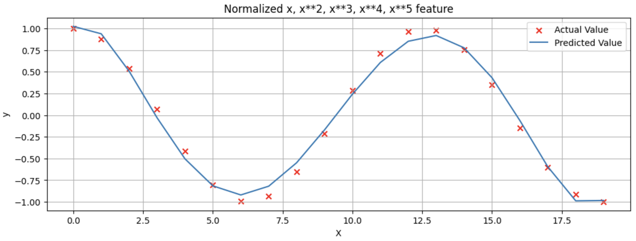
plt.figure(figsize=(12, 4))
plt.scatter(x, y, marker='x', c='r', label="Actual Value"); plt.title("Normalized x x**2, x**3, x**4, x**5 feature")
plt.plot(x, X@w_final + b_final, label="Predicted Value");  plt.xlabel("X"); plt.ylabel("y")
plt.legend()
plt.grid()
plt.show()

执行结果

参考

吴恩达团队在Coursera开设的机器学习课程：https://www.coursera.org/specializations/machine-learning-introduction

在B站学习：https://www.bilibili.com/video/BV1Pa411X76s