统计学习方法---感知机模型

作业:

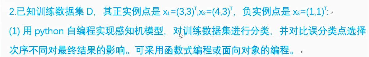
一:感知机算法原始形式实现

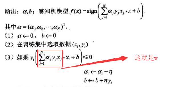
（一）伪代码

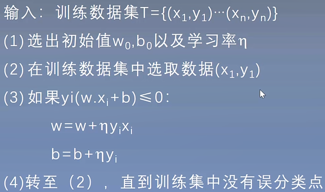
（二）实现感知机算法

class MyPerceptron:
    def __init__(self):  # 属性初始化
        self.w = None
        self.b = 0
        self.l_rate = 1

    def fit(self, X_train, y_train):
        global history_w, history_b　　#保持w,b信息，方便一会绘制图像
        # 根据X形状,设置w
        self.w = np.zeros(X_train.shape[1])
        i = 0

        while i < X_train.shape[0]:  # 注意我们按顺序查看误分类点
            X = X_train[i]
            y = y_train[i]
            # 如果y*(wX+b)<=0,则是误分类点,我们就要更新一次w,b,我们每更新一次w,b,我们就要从新查找整个数据集
            if y * (np.dot(self.w, X) + self.b) <= 0:
                self.w = self.w + self.l_rate * np.dot(y, X)
                self.b = self.b + self.l_rate * y
                i = 0
                history_w.append(self.w)
                history_b.append(self.b)
            else:
                i += 1

（三）设置数据，进行训练

if __name__ == "__main__":
    # 构建数据集和标签值
    X_train = np.array([[3, 3], [4, 3], [1, 1]])
    y = np.array([1, 1, -1])
    history_w = []
    history_b = []

    perc = MyPerceptron()
    perc.fit(X_train, y)  # 进行训练 获取w,b信息

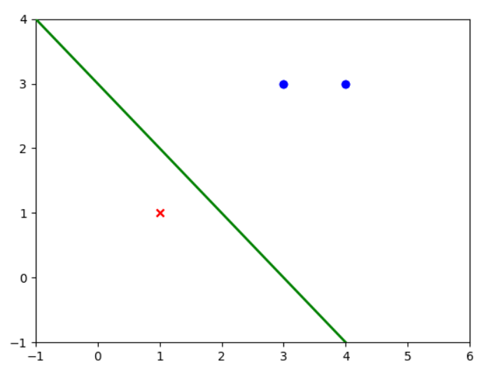
（四）数据可视化

    # 数据集可视化
    fig = plt.figure()
    ax = plt.axes()
    line, = ax.plot([], [], 'g', lw=2)


    def init():
        line.set_data([], [])
        plt.scatter(X_train[np.where(y == 1), 0], X_train[np.where(y == 1), 1], marker="o", c="b")
        plt.scatter(X_train[np.where(y == -1), 0], X_train[np.where(y == -1), 1], marker="x", c="r")
        return line,

    def update(i):
        global history_w, history_b, ax, line
        w = history_w[i]
        b = history_b[i]
        if w[1] == 0:
            return line,

        x1 = -1
        y1 = -(b + w[0] * x1) / w[1]

        x2 = 6
        y2 = -(b + w[0] * x2) / w[1]

        line.set_data([x1, x2], [y1, y2])

        return line,

    plt.xlim(-1, 6)
    plt.ylim(-1, 4)

    print(history_w)
    print(history_b)
    #[[[3, 3], 1], [[2, 2], 0], [[1, 1], -1], [[0, 0], -2], [[3, 3], -1], [[2, 2], -2], [[1, 1], -3]]
    ani = anim.FuncAnimation(fig=fig, func=update,init_func=init, frames=len(history_b), interval=1000, repeat=True, blit=True)

    plt.show()

参数详解：

1. fig 进行动画绘制的figure
2. func 自定义动画函数，即传入刚定义的函数animate
3. frames 动画长度，一次循环包含的帧数
4. init_func 自定义开始帧，即传入刚定义的函数init
5. interval 更新频率，以ms计
6. blit 选择更新所有点，还是仅更新产生变化的点。应选择True，但mac用户请选择False，否则无法显示动画

注意：我们要实现Animation动画，需要设置pycharm中(File->Settings->Tools->Python Scientific）的Show plots in tool window选项（disable不使用）

（五）结果显示

import numpy as np
import matplotlib.pyplot as plt
import matplotlib.animation as anim


class MyPerceptron:
    def __init__(self):  # 属性初始化
        self.w = None
        self.b = 0
        self.l_rate = 1

    def fit(self, X_train, y_train):
        global history_w, history_b
        # 根据X形状,设置w
        self.w = np.zeros(X_train.shape[1])
        i = 0

        while i < X_train.shape[0]:  # 注意我们按顺序查看误分类点
            X = X_train[i]
            y = y_train[i]
            # 如果y*(wX+b)<=0,则是误分类点,我们就要更新一次w,b,我们每更新一次w,b,我们就要从新查找整个数据集
            if y * (np.dot(self.w, X) + self.b) <= 0:
                self.w = self.w + self.l_rate * np.dot(y, X)
                self.b = self.b + self.l_rate * y
                i = 0
                history_w.append(self.w)
                history_b.append(self.b)
            else:
                i += 1


if __name__ == "__main__":
    # 构建数据集和标签值
    X_train = np.array([[3, 3], [4, 3], [1, 1]])
    y = np.array([1, 1, -1])
    history_w = []
    history_b = []

    perc = MyPerceptron()
    perc.fit(X_train, y)  # 进行训练 获取w,b信息

    # 数据集可视化
    fig = plt.figure()
    ax = plt.axes()
    line, = ax.plot([], [], 'g', lw=2)


    def init():
        line.set_data([], [])
        plt.scatter(X_train[np.where(y == 1), 0], X_train[np.where(y == 1), 1], marker="o", c="b")
        plt.scatter(X_train[np.where(y == -1), 0], X_train[np.where(y == -1), 1], marker="x", c="r")
        return line,

    def update(i):
        global history_w, history_b, ax, line
        w = history_w[i]
        b = history_b[i]
        if w[1] == 0:
            return line,

        x1 = -1
        y1 = -(b + w[0] * x1) / w[1]

        x2 = 6
        y2 = -(b + w[0] * x2) / w[1]

        line.set_data([x1, x2], [y1, y2])

        return line,

    plt.xlim(-1, 6)
    plt.ylim(-1, 4)

    print(history_w)
    print(history_b)
    #[[[3, 3], 1], [[2, 2], 0], [[1, 1], -1], [[0, 0], -2], [[3, 3], -1], [[2, 2], -2], [[1, 1], -3]]
    ani = anim.FuncAnimation(fig=fig, func=update,init_func=init, frames=len(history_b), interval=1000, repeat=True, blit=True)

    plt.show()

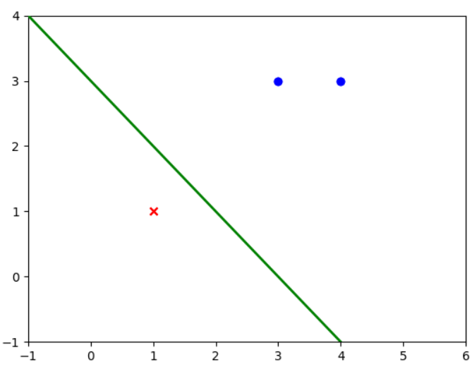
二：感知机算法对偶形式实现

（一）伪代码

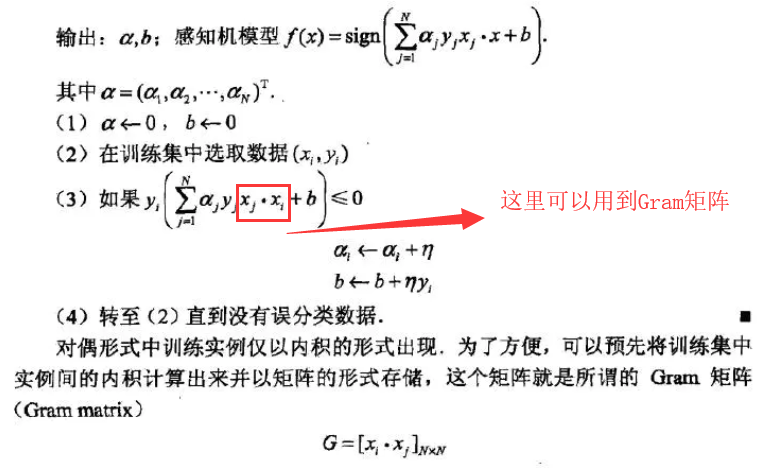
（二）实现感知机对偶算法

class MyPerceptron:
    def __init__(self):  # 属性初始化
        self.a = None
        self.b = 0
        self.l_rate = 1
        self.gram = None
        self.gram_diag = None

    def cal_gram(self,X_train):
        self.gram = np.zeros((X_train.shape[0],X_train.shape[0]))
        self.gram = np.dot(X_train,X_train.T)

    def fit(self, X_train, y_train):
        global history_a, history_b
        self.cal_gram(X_train)
        # 根据X形状,设置a  对于每一个样本，都有一个a
        self.a = np.zeros(X_train.shape[0])
        i = 0

        while i < X_train.shape[0]:  # 注意我们按顺序查看误分类点
            y = y_train[i]
            sigma_gram = np.sum(self.gram[i]*self.a*y_train)    #使用了gram矩阵，减少计算量
            # 如果y*(wX+b)<=0,则是误分类点,我们就要更新一次w,b,我们每更新一次w,b,我们就要从新查找整个数据集
            if y * (sigma_gram + self.b) <= 0:
                self.a[i] = self.a[i]+ self.l_rate
                self.b = self.b + self.l_rate * y
                i = 0
                history_a.append(self.a.copy())
                history_b.append(self.b)
            else:
                i += 1

（三）训练数据

if __name__ == "__main__":
    # 构建数据集和标签值
    X_train = np.array([[3, 3], [4, 3], [1, 1]])
    y_train = np.array([1, 1, -1])
    history_a = []
    history_b = []

    perc = MyPerceptron()
    perc.fit(X_train, y_train)  # 进行训练 获取w,b信息

    # 数据集可视化
    fig = plt.figure()
    ax = plt.axes()
    line, = ax.plot([], [], 'g', lw=2)
    print(history_a)
    print(history_b)

（四）数据可视化

if __name__ == "__main__":
    # 构建数据集和标签值
    X_train = np.array([[3, 3], [4, 3], [1, 1]])
    y_train = np.array([1, 1, -1])
    history_a = []
    history_b = []

    perc = MyPerceptron()
    perc.fit(X_train, y_train)  # 进行训练 获取w,b信息

    # 数据集可视化
    fig = plt.figure()
    ax = plt.axes()
    line, = ax.plot([], [], 'g', lw=2)
    print(history_a)
    print(history_b)

    def init():
        line.set_data([], [])
        plt.scatter(X_train[np.where(y_train == 1), 0], X_train[np.where(y_train == 1), 1], marker="o", c="b")
        plt.scatter(X_train[np.where(y_train == -1), 0], X_train[np.where(y_train == -1), 1], marker="x", c="r")
        return line,

    def update(i):
        global history_a, history_b, line,X_train,y_train
        a = history_a[i]
        b = history_b[i]

        w = np.sum(X_train*np.array([a]).T*np.array([y_train]).T,0) #这一步实现获取w

        if w[1] == 0:
            return line,

        x1 = -1
        y1 = -(b + w[0] * x1) / w[1]

        x2 = 6
        y2 = -(b + w[0] * x2) / w[1]

        line.set_data([x1, x2], [y1, y2])

        return line,

    plt.xlim(-1, 6)
    plt.ylim(-1, 4)

    ani = anim.FuncAnimation(fig=fig, func=update,init_func=init, frames=len(history_b), interval=1000, repeat=True, blit=True)

    plt.show()

（五）结果显示

import numpy as np
import matplotlib.pyplot as plt
import matplotlib.animation as anim

class MyPerceptron:
    def __init__(self):  # 属性初始化
        self.a = None
        self.b = 0
        self.l_rate = 1
        self.gram = None
        self.gram_diag = None

    def cal_gram(self,X_train):
        self.gram = np.zeros((X_train.shape[0],X_train.shape[0]))
        self.gram = np.dot(X_train,X_train.T)

    def fit(self, X_train, y_train):
        global history_a, history_b
        self.cal_gram(X_train)
        # 根据X形状,设置a  对于每一个样本，都有一个a
        self.a = np.zeros(X_train.shape[0])
        i = 0

        while i < X_train.shape[0]:  # 注意我们按顺序查看误分类点
            y = y_train[i]
            sigma_gram = np.sum(self.gram[i]*self.a*y_train)    #使用了gram矩阵，减少计算量
            # 如果y*(wX+b)<=0,则是误分类点,我们就要更新一次w,b,我们每更新一次w,b,我们就要从新查找整个数据集
            if y * (sigma_gram + self.b) <= 0:
                self.a[i] = self.a[i]+ self.l_rate
                self.b = self.b + self.l_rate * y
                i = 0
                history_a.append(self.a.copy())
                history_b.append(self.b)
            else:
                i += 1

if __name__ == "__main__":
    # 构建数据集和标签值
    X_train = np.array([[3, 3], [4, 3], [1, 1]])
    y_train = np.array([1, 1, -1])
    history_a = []
    history_b = []

    perc = MyPerceptron()
    perc.fit(X_train, y_train)  # 进行训练 获取w,b信息

    # 数据集可视化
    fig = plt.figure()
    ax = plt.axes()
    line, = ax.plot([], [], 'g', lw=2)
    print(history_a)
    print(history_b)

    def init():
        line.set_data([], [])
        plt.scatter(X_train[np.where(y_train == 1), 0], X_train[np.where(y_train == 1), 1], marker="o", c="b")
        plt.scatter(X_train[np.where(y_train == -1), 0], X_train[np.where(y_train == -1), 1], marker="x", c="r")
        return line,

    def update(i):
        global history_a, history_b, line,X_train,y_train
        a = history_a[i]
        b = history_b[i]

        w = np.sum(X_train*np.array([a]).T*np.array([y_train]).T,0)
        print(w,b)

        if w[1] == 0:
            return line,

        x1 = -1
        y1 = -(b + w[0] * x1) / w[1]

        x2 = 6
        y2 = -(b + w[0] * x2) / w[1]

        line.set_data([x1, x2], [y1, y2])

        return line,

    plt.xlim(-1, 6)
    plt.ylim(-1, 4)

    ani = anim.FuncAnimation(fig=fig, func=update,init_func=init, frames=len(history_b), interval=1000, repeat=True, blit=True)

    plt.show()

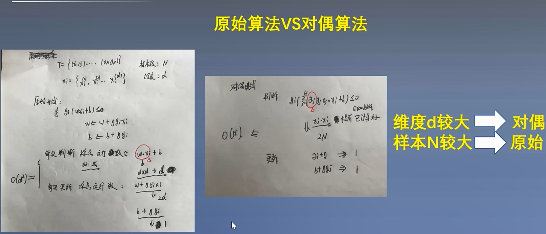
（六）原始算法对比对偶算法

三：Sklearn实现感知机

（一）代码实现

import numpy as np
import matplotlib.pyplot as plt
from sklearn.linear_model import Perceptron

if __name__ == "__main__":
    # 构建数据集和标签值
    X_train = np.array([[3, 3], [4, 3], [1, 1]])
    y_train = np.array([1, 1, -1])
    #构建Perceptron对象，训练数据并输出结果
    perc = Perceptron()
    perc.fit(X_train,y_train)
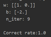
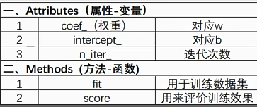
    print("w:",perc.coef_,"\n","b:",perc.intercept_,"\n","n_iter:",perc.n_iter_,"\n")
    #获取模型预测的准确率
    res = perc.score(X_train,y_train)
    print("Correct rate:{}".format(res))

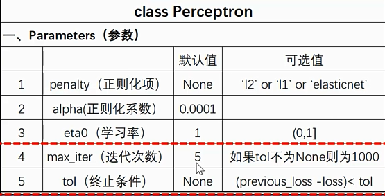
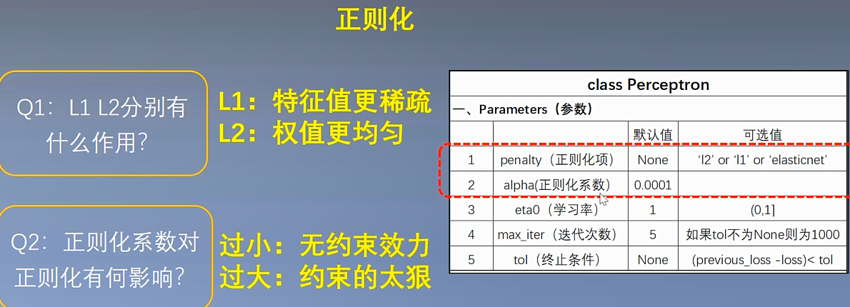
（二）方法参数说明