PINN: Time-dependent 1D problem

Problem Description

Suppose we have a simple partial differential equation as follows.

\[\frac{1}{2}\frac{\partial u}{\partial t}=\frac{\partial^2u}{\partial x^2},\quad u(x,0)=\sin(\pi x) \]

If we look into another equation (2), you can see this is one of the possible solutions of (1).

\[u(x,t)=e^{-2\pi^2t}\sin(\pi x) \]

Now we will use (2) to create training dataset, build custom loss function according to the concept of PINN, train our model with or without PINN concept.

Training Data Generation

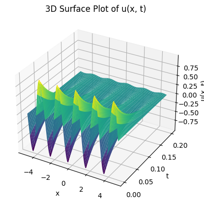
Let’s create our training data first. The sampling domain was set to be \((x,t)\in[-5,5]\times[0,0.2]\)

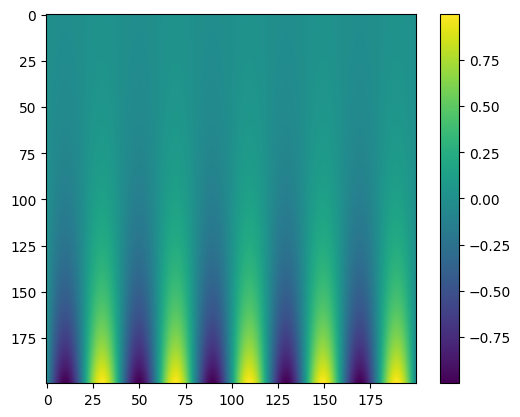
The 3D plot:

Ordinary Neural Network

Neural Network Architecture: (indim, 100, outdim)
Activation Function: Tanh
Optimization Algorithm: Adam(Learning Rate = 0.1)
Loss Function: MSE
Epochs: 500
Final: Saving model with loss 0.0033...

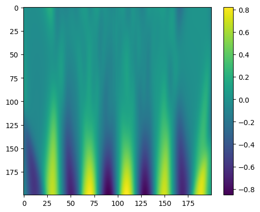
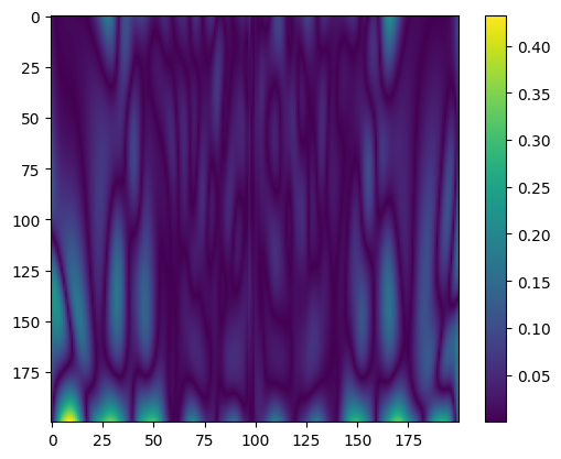
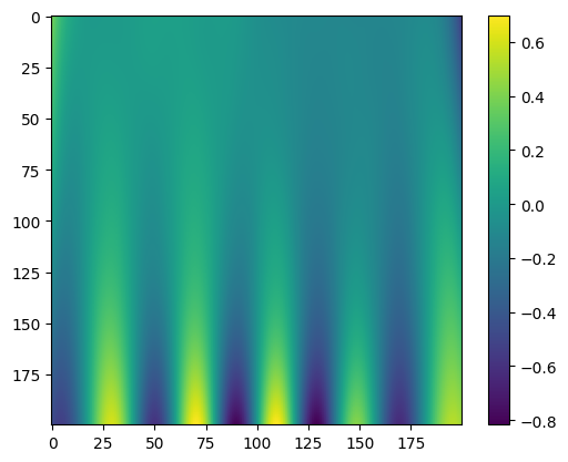
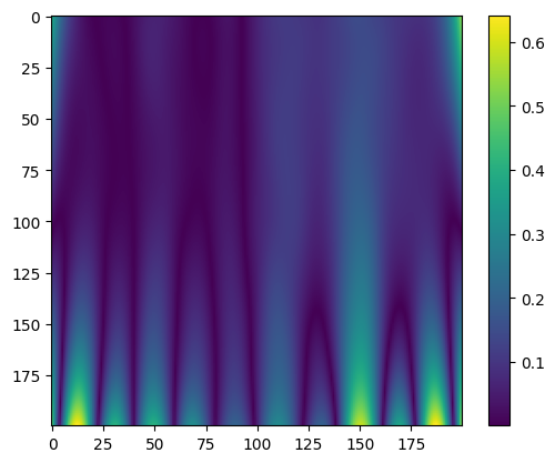
Predicted value	Error

PINN

Neural Network Architecture: (indim, 100, outdim)
Activation Function: Tanh
Optimization Algorithm: Adam(Learning Rate = 0.1)
Loss Function: MSE + Physical and boundary losses
Epochs: 500
Final: Saving model with loss 0.1832...

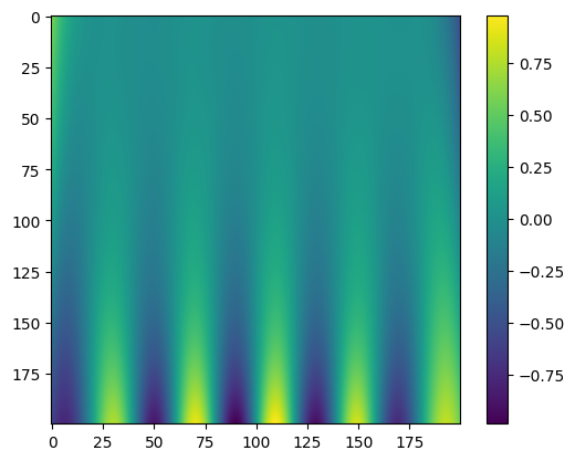
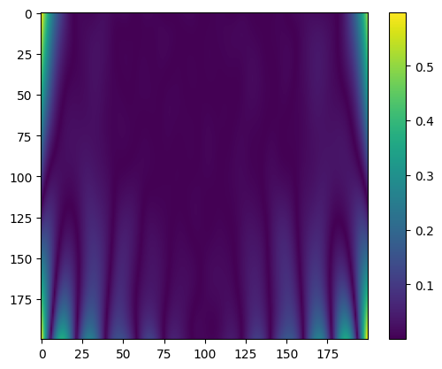
Predicted value	Error

PINN with LBFGS

Neural Network Architecture: (indim, 100, outdim)
Activation Function: Tanh
Optimization Algorithm: Adam(Learning Rate = 0.1), LBFGS(Learning Rate = 0.01)
Loss Function: MSE + Physical and boundary losses
Epochs: 200(Adam), 30(LBFGS)
Final: Saving model with loss 0.0824...

Predicted value	Error

Conclusion

Using PINN can achieve good results faster within the same number of iterations. The LBFGS optimization algorithm can further optimize the loss based on Adam and achieve better results, but the running speed will be much slower than Adam.

Code

https://github.com/srrdhy/PINN_Tutorial

Reference

https://lazyjobseeker.github.io/en/posts/physics-informed-neural-network-tutorials/#training-model-with-pinn