Regularization —— linear regression
本节主要是练习regularization项的使用原则。因为在机器学习的一些模型中,如果模型的参数太多,而训练样本又太少的话,这样训练出来的模型很容易产生过拟合现象。因此在模型的损失函数中,需要对模型的参数进行“惩罚”,这样的话这些参数就不会太大,而越小的参数说明模型越简单,越简单的模型则越不容易产生过拟合现象。
Regularized linear regression
From looking at this plot, it seems that fitting a straight line might be too simple of an approximation. Instead, we will try fitting a higher-order polynomial to the data to capture more of the variations in the points.
Let's try a fifth-order polynomial. Our hypothesis will be
![]()
This means that we have a hypothesis of six features, because ![]() are now all features of our regression. Notice that even though we are producing a polynomial fit, we still have a linear regression problem because the hypothesis is linear in each feature.
are now all features of our regression. Notice that even though we are producing a polynomial fit, we still have a linear regression problem because the hypothesis is linear in each feature.
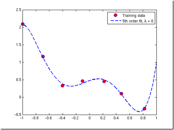
Since we are fitting a 5th-order polynomial to a data set of only 7 points, over-fitting is likely to occur. To guard against this, we will use regularization in our model.
Recall that in regularization problems, the goal is to minimize the following cost function with respect to ![]() :
:

The regularization parameter ![]() is a control on your fitting parameters. As the magnitues of the fitting parameters increase, there will be an increasing penalty on the cost function. This penalty is dependent on the squares of the parameters as well as the magnitude of
is a control on your fitting parameters. As the magnitues of the fitting parameters increase, there will be an increasing penalty on the cost function. This penalty is dependent on the squares of the parameters as well as the magnitude of ![]() . Also, notice that the summation after
. Also, notice that the summation after ![]() does not include
does not include ![]()
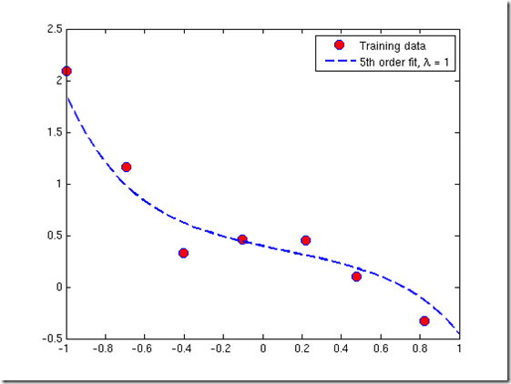
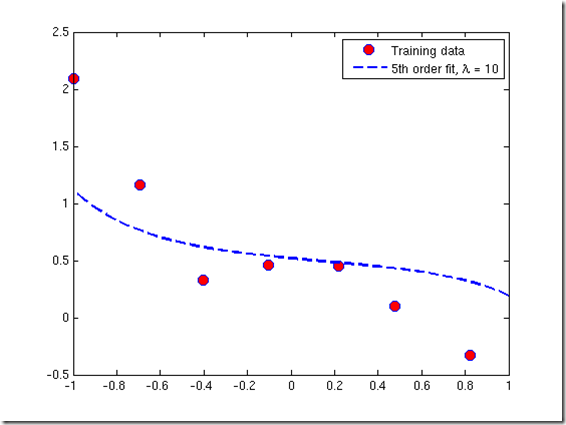
lamda 越大,训练出的模型越简单 —— 后一项的惩罚越大
Normal equations
Now we will find the best parameters of our model using the normal equations. Recall that the normal equations solution to regularized linear regression is
The matrix following
is an
diagonal matrix with a zero in the upper left and ones down the other diagonal entries. (Remember that
is the number of features, not counting the intecept term). The vector
and the matrix
have the same definition they had for unregularized regression:
Using this equation, find values for
using the three regularization parameters below:
a.
(this is the same case as non-regularized linear regression)
b.
c.
Code
clc,clear
%加载数据
x = load('ex5Linx.dat');
y = load('ex5Liny.dat');

%显示原始数据
plot(x,y,'o','MarkerEdgeColor','b','MarkerFaceColor','r')

%将特征值变成训练样本矩阵
x = [ones(length(x),1) x x.^2 x.^3 x.^4 x.^5];
[m n] = size(x);
n = n -1;

%计算参数sidta,并且绘制出拟合曲线
rm = diag([0;ones(n,1)]);%lamda后面的矩阵
lamda = [0 1 10]';
colortype = {'g','b','r'};
sida = zeros(n+1,3); %初始化参数sida
xrange = linspace(min(x(:,2)),max(x(:,2)))';
hold on;
for i = 1:3
    sida(:,i) = inv(x'*x+lamda(i).*rm)*x'*y;%计算参数sida
    norm_sida = norm(sida) % norm 求sida的2阶范数
    yrange = [ones(size(xrange)) xrange xrange.^2 xrange.^3,...
        xrange.^4 xrange.^5]*sida(:,i);
    plot(xrange',yrange,char(colortype(i)))
    hold on
end
legend('traning data', '\lambda=0', '\lambda=1','\lambda=10')%注意转义字符的使用方法
hold off


![\begin{displaymath}
\theta=(X^{T}X+\lambda\left[\begin{array}{cccc}
0\\
& 1\\
& & \ddots\\
& & & 1\end{array}\right])^{-1}X^{T}\vec{y}\end{displaymath}](http://openclassroom.stanford.edu/MainFolder/courses/DeepLearning/exercises/ex5/img7.png)
![\begin{displaymath}
\begin{array}{cc}
\par
\vec{y} = \left[
\begin{array}{c}
y...
...m)})^T\mbox{-}
\end{array}\right] \nonumber
\par
\end{array}\end{displaymath}](http://openclassroom.stanford.edu/MainFolder/courses/DeepLearning/exercises/ex5/img12.png)


 浙公网安备 33010602011771号