

详细介绍:线性代数 | Graphic Notes on “Linear Algebra for Everyone”
注:本文为 “The Art of Linear Algebra 重排版” 。
英文引文,机翻未校。
如有内容异常,请看原文。
The Art of Linear Algebra
Graphic Notes on “Linear Algebra for Everyone”
Kenji Hiranabe *
with the kindest help of Gilbert Strang †
translator: Kefang Liu ‡
September 1, 2021/updated August 19, 2023
线性代数的艺术
摘要
我尝试为吉尔伯特·斯特朗(Gilbert Strang)在《人人都懂线性代数》(“Linear Algebra for Everyone”)一书中介绍的矩阵重要概念进行可视化图解,以促进从矩阵分解的角度对向量、矩阵计算和算法的理解。这些概念包括矩阵分解(列 - 行分解,Column - Row, CR)、高斯消去法(Gaussian Elimination, LU)、格拉姆 - 施密特正交化(Gram - Schmidt Orthogonalization, QR)、特征值与对角化(Eigenvalues and Diagonalization,Q Λ Q T Q\Lambda Q^TQΛQT)以及奇异值分解(Singular Value Decomposition,U Σ V T U\Sigma V^TUΣVT)。
序言
我很高兴能看到 Kenji Hiranabe 关于线性代数中矩阵运算的图解!这样的图解是展示代数的绝佳方式。我们固然可以通过行 · 列的点乘来理解矩阵乘法,但这绝非全部——矩阵乘法是由“线性组合”与“秩 1 矩阵”共同构成的代数与艺术。我很感激能看到这本书的日文翻译版本以及 Kenji Hiranabe 图解中所蕴含的思想。
——吉尔伯特·斯特朗(Gilbert Strang)
麻省理工学院数学教授
- twitter:@hiranabe, k-hiranabe@esm.co.jp,https://anagileway.com
† Massachusetts Institute of Technology,http://www-math.mit.edu/~gs/
‡ twitter:@kfcliu, 微博用户: 5717297833
“Linear Algebra for Everyone”:http://math.mit.edu/everyone/
1 理解矩阵——4 个视角
一个矩阵可以被视为 1 个矩阵、m × n m\times nm×n 个元素、n nn 个列向量和 m mm 个行向量。
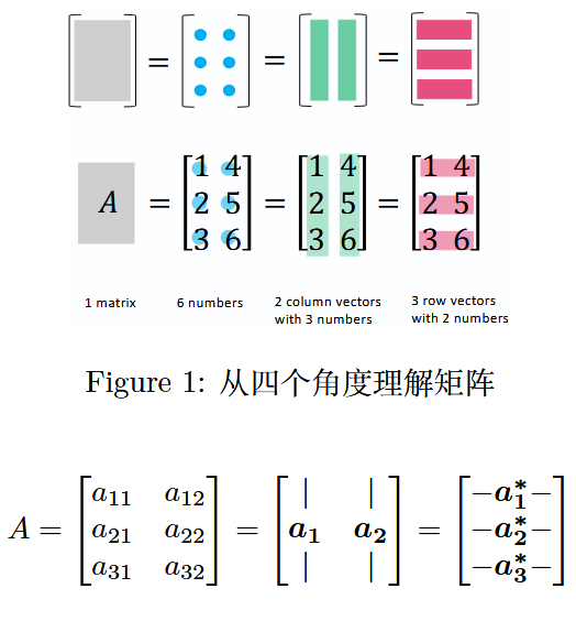
图 1:从四个角度理解矩阵
在这里,列向量被标记为粗体a j a_jaj;行向量则有一个∗ *∗ 号,标记为 a i ∗ a_i^*ai∗;转置向量和矩阵则用T TT 标记为 a j T a_j^TajT 和 A T A^TAT。
2 向量乘以向量——2 个视角
在后文中,我将介绍一些概念,同时列出《人人都懂线性代数》(“Linear Algebra for Everyone”)一书中的相应部分(部分编号插入如下)。详细内容建议参考原书,此处我也添加了简短解释,以便您能通过本文尽可能多地理解相关知识。此外,每个图都有一个简短名称,例如v 1 v1v1(数字 1 表示向量的乘积)、M v 1 Mv1Mv1(数字 1 表示矩阵和向量的乘积),以及如下图(v 1 v1v1)所示的彩色圆圈。随着讨论的推进,会对该名称进行交叉引用。
- 1.1 节(p.2)线性组合与点积(Linear combination and dot products)
- 1.3 节(p.25)秩 1 矩阵(Matrix of Rank One)
- 1.4 节(p. 29)行视角与列视角(Row way and column way)
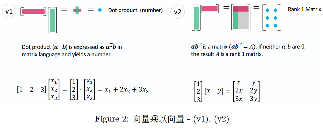
图 2:向量乘以向量 -(v 1 v1v1),(v 2 v2v2)
(v 1 v1v1)是两个向量之间的基础运算,即向量内积;而(v 2 v2v2)是将列向量乘以行向量,从而产生一个秩 1 矩阵。
理解(v 2 v2v2)的结果(秩 1 矩阵)是后续章节的关键。
3 矩阵乘以向量——2 个视角
一个矩阵乘以一个向量,会产生由三个点积组成的向量(M v 1 Mv1Mv1),同时也是矩阵列向量的一种线性组合(M v 2 Mv2Mv2)。
- 1.1 节(p. 3)线性组合(Linear combinations)
- 1.3 节(p. 21)矩阵与列空间(Matrices and Column Spaces)
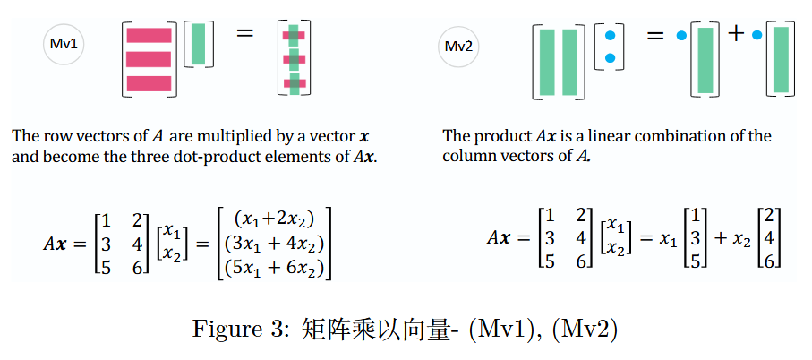
图 3:矩阵乘以向量 -(M v 1 Mv1Mv1),(M v 2 Mv2Mv2)
通常,人们会先学习(M v 1 Mv1Mv1)此种矩阵乘向量的视角。但当你习惯从(M v 2 Mv2Mv2)的视角看待矩阵乘向量时,会理解到A x AxAx 是矩阵 A AA列向量的线性组合。矩阵A AA的列向量的所有线性组合生成的子空间记为C ( A ) C(A)C(A)(列空间),A x = 0 Ax = 0Ax=0的解空间则是零空间,记为N ( A ) N(A)N(A)。
同理,由(v M 1 vM1vM1)和(v M 2 vM2vM2)可知,行向量乘以矩阵也可以用类似的方式理解。
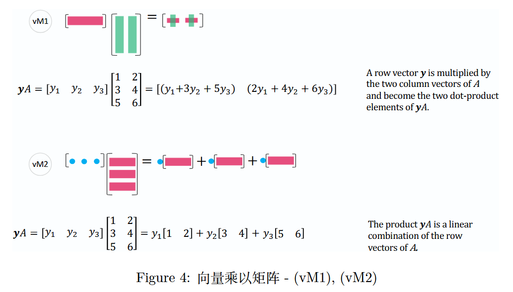
图 4:向量乘以矩阵 -(v M 1 vM1vM1),(v M 2 vM2vM2)
上图中,矩阵A AA的行向量的所有线性组合生成的子空间记为C ( A T ) C(A^T)C(AT)(行空间),y T A = 0 y^T A = 0yTA=0 的解空间是 A AA的左零空间,记为N ( A T ) N(A^T)N(AT)。
Row Vector Multiplication with MatrixA AA
矩阵 A AA的行向量乘法A row vectory yyis multiplied by the two column vectors ofA AAand become the two dot-product elements ofy A yAyA.
行向量 y yy 与矩阵 A AA的两个列向量相乘,成为y A yAyA的两个点积元素。y A = [ y 1 y 2 y 3 ] [ 1 2 3 4 5 6 ] = [ ( y 1 + 3 y 2 + 5 y 3 ) ( 2 y 1 + 4 y 2 + 6 y 3 ) ] yA = \begin{bmatrix} y_1 & y_2 & y_3 \end{bmatrix} \begin{bmatrix} 1 & 2 \\ 3 & 4 \\ 5 & 6 \end{bmatrix} = \begin{bmatrix} (y_1 + 3y_2 + 5y_3) & (2y_1 + 4y_2 + 6y_3) \end{bmatrix}yA=[y1y2y3]135246=[(y1+3y2+5y3)(2y1+4y2+6y3)]
行向量 y yy 与矩阵 A AA相乘,结果是一个新行向量,它由y yy 与 A AA的每个列向量的点积形成。
Linear Combination of Row Vectors of MatrixA AA
矩阵 A AA的行向量的线性组合The producty A yAyAis a linear combination of the row vectors ofA AA.
乘积 y A yAyA 是矩阵 A AA行向量的线性组合。y A = [ y 1 y 2 y 3 ] [ 1 2 3 4 5 6 ] = y 1 [ 1 2 ] + y 2 [ 3 4 ] + y 3 [ 5 6 ] yA = \begin{bmatrix} y_1 & y_2 & y_3 \end{bmatrix} \begin{bmatrix} 1 & 2 \\ 3 & 4 \\ 5 & 6 \end{bmatrix} = y_1 \begin{bmatrix} 1 & 2 \end{bmatrix} + y_2 \begin{bmatrix} 3 & 4 \end{bmatrix} + y_3 \begin{bmatrix} 5 & 6 \end{bmatrix}yA=[y1y2y3]135246=y1[12]+y2[34]+y3[56]
行向量 y yy 与矩阵 A AA的乘积得到的新向量是A AA的行向量的线性组合。
本书的一大亮点是介绍了四个基本子空间:在R n \mathbb{R}^nRn 上的 C ( A ) C(A)C(A)(列空间)和N ( A T ) N(A^T)N(AT)(左零空间)(相互正交),以及在R m \mathbb{R}^mRm 上的 C ( A T ) C(A^T)C(AT)(行空间)和N ( A ) N(A)N(A)(零空间)(相互正交)。
- 3.5 节(p. 124)四个子空间的维数(Dimensions of the Four Subspaces)
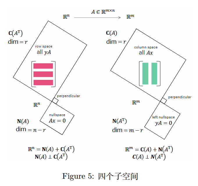
图 5:四个子空间
关于秩 r rr,请见(6.1 节)A = C R A = CRA=CR 分解。
4 矩阵乘以矩阵——4 个视角
由“矩阵乘以向量”可自然延伸到“矩阵乘以矩阵”。
- 1.4 节(p. 35)矩阵乘法的四种方式(Four ways to multiply)
- 也可参考原书封底
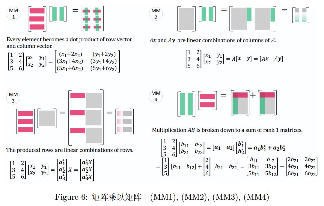
图 6:矩阵乘以矩阵 -(M M 1 MM1MM1),(M M 2 MM2MM2),(M M 3 MM3MM3),(M M 4 MM4MM4)
第一种方式(按元素计算):
Every element becomes a dot product of row vector and column vector.
每个元素都变成行向量和列向量的点积。
[ 1 2 3 4 5 6 ] [ x 1 y 1 x 2 y 2 ] = [ ( x 1 + 2 x 2 ) ( y 1 + 2 y 2 ) ( 3 x 1 + 4 x 2 ) ( 3 y 1 + 4 y 2 ) ( 5 x 1 + 6 x 2 ) ( 5 y 1 + 6 y 2 ) ] \begin{bmatrix}1&2\\3&4\\5&6\end{bmatrix}\begin{bmatrix}x_1&y_1\\x_2&y_2\end{bmatrix}=\begin{bmatrix}(x_1 + 2x_2)&(y_1 + 2y_2)\\(3x_1 + 4x_2)&(3y_1 + 4y_2)\\(5x_1 + 6x_2)&(5y_1 + 6y_2)\end{bmatrix}135246[x1x2y1y2]=(x1+2x2)(3x1+4x2)(5x1+6x2)(y1+2y2)(3y1+4y2)(5y1+6y2)
第二种方式(按列组合):
A x AxAx and A y AyAyare linear combinations of columns ofA AA.
A x AxAx 和 A y AyAy 是矩阵 A AA列向量的线性组合。
[ 1 2 3 4 5 6 ] [ x 1 y 1 x 2 y 2 ] = A [ x y ] = [ A x A y ] \begin{bmatrix}1&2\\3&4\\5&6\end{bmatrix}\begin{bmatrix}x_1&y_1\\x_2&y_2\end{bmatrix}=A\begin{bmatrix}x&y\end{bmatrix}=\begin{bmatrix}Ax&Ay\end{bmatrix}135246[x1x2y1y2]=A[xy]=[AxAy]
第三种方式(按行组合):
The produced rows are linear combinations of rows.
行的线性组合。就是产生的行
[ 1 2 3 4 5 6 ] [ x 1 y 1 x 2 y 2 ] = [ a 1 ∗ a 2 ∗ a 3 ∗ ] X = [ a 1 ∗ X a 2 ∗ X a 3 ∗ X ] \begin{bmatrix} 1 & 2 \\ 3 & 4 \\ 5 & 6 \end{bmatrix} \begin{bmatrix} x_1 & y_1 \\ x_2 & y_2 \end{bmatrix} = \begin{bmatrix} a_1^* \\ a_2^* \\ a_3^* \end{bmatrix} X = \begin{bmatrix} a_1^*X \\ a_2^*X \\ a_3^*X \end{bmatrix}135246[x1x2y1y2]=a1∗a2∗a3∗X=a1∗Xa2∗Xa3∗X
其中,a i ∗ X a_i^*Xai∗X 是矩阵 X XX行向量的线性组合。
第四种方式(秩 1 矩阵求和):
Matrix Multiplication as a Sum of Rank 1 Matrices.
矩阵乘法可分解为若干个秩 1 矩阵之和,即A B = ∑ k = 1 n a k b k ∗ AB=\sum_{k = 1}^n a_k b_k^*AB=∑k=1nakbk∗,其中 a k a_kak 是矩阵 A AA 的第 k kk 列,b k ∗ b_k^*bk∗ 是矩阵 B BB 的第 k kk 行。
Matrix multiplicationA B ABABis broken down to a sum of rank 1 matrices.
矩阵乘法 A B ABAB被分解为秩为 1 的矩阵之和。
[ 1 2 3 4 5 6 ] [ b 11 b 12 b 21 b 22 ] = [ a 1 a 2 ] [ b 1 ∗ b 2 ∗ ] = a 1 b 1 ∗ + a 2 b 2 ∗ = [ 1 3 ] [ b 11 b 12 ] + [ 2 4 ] [ b 21 b 22 ] = [ b 11 b 12 3 b 11 3 b 12 5 b 11 5 b 12 ] + [ 2 b 21 2 b 22 4 b 21 4 b 22 6 b 21 6 b 22 ] \begin{align*} \left[ \begin{matrix} 1 & 2 \\ 3 & 4 \\ 5 & 6 \end{matrix} \right] \left[ \begin{matrix} b_{11} & b_{12} \\ b_{21} & b_{22} \end{matrix} \right] &= \left[ \begin{matrix} a_1 & a_2 \end{matrix} \right] \left[ \begin{matrix} b_1^* \\ b_2^* \end{matrix} \right] &=& a_1 b_1^* + a_2 b_2^* \\ &= \left[ \begin{matrix} 1 \\ 3 \end{matrix} \right] \left[ \begin{matrix} b_{11} & b_{12} \end{matrix} \right] + \left[ \begin{matrix} 2 \\ 4 \end{matrix} \right] \left[ \begin{matrix} b_{21} & b_{22} \end{matrix} \right] &=& \left[ \begin{matrix} b_{11} & b_{12} \\ 3b_{11} & 3b_{12} \\ 5b_{11} & 5b_{12} \end{matrix} \right] + \left[ \begin{matrix} 2b_{21} & 2b_{22} \\ 4b_{21} & 4b_{22} \\ 6b_{21} & 6b_{22} \end{matrix} \right] \end{align*}135246[b11b21b12b22]=[a1a2][b1∗b2∗]=[13][b11b12]+[24][b21b22]==a1b1∗+a2b2∗b113b115b11b123b125b12+2b214b216b212b224b226b22
5 实用模式
在这里,我将展示一些实用模式,帮助你更直观地理解后续内容。
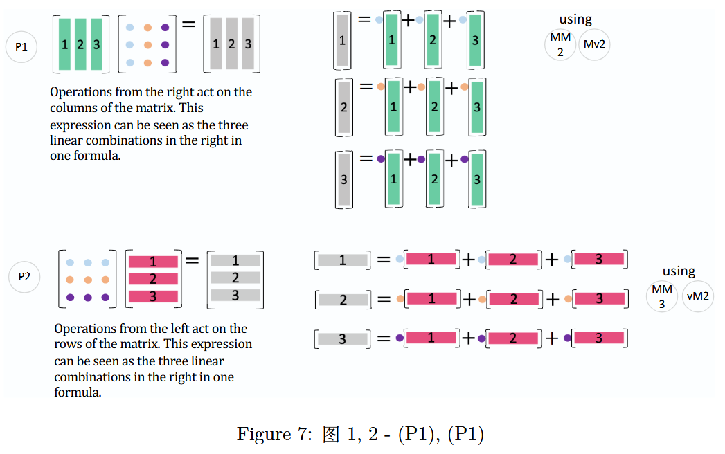
图 7:图 1,2 -(P 1 P1P1),(P 2 P2P2)
Matrix Operations: Right and Left Multiplications
矩阵运算:右乘和左乘P 1 P1P1 是(M M 2 MM2MM2)(矩阵乘矩阵的列组合方式)和(M v 2 Mv2Mv2)(矩阵乘向量的列组合方式)的结合。
Operations from the right act on the columns of the matrix. This expression can be seen as the three linear combinations in the right in one formula.
通过右侧操控作用于矩阵的列。该表达式能够看作是一个公式中的三个线性组合。P 2 P2P2 是(M M 3 MM3MM3)(矩阵乘矩阵的行组合方式)和(v M 2 vM2vM2)(向量乘矩阵的行组合方式)的扩展。
Operations from the left act on the rows of the matrix. This expression can be seen as the three linear combinations in the right in one formula.
左侧操作作用于矩阵的行。这个表达式可以看作是一个公式中的三个线性组合。
需要注意的是,P 1 P1P1对应列运算(右乘一个矩阵),而P 2 P2P2对应行运算(左乘一个矩阵)。
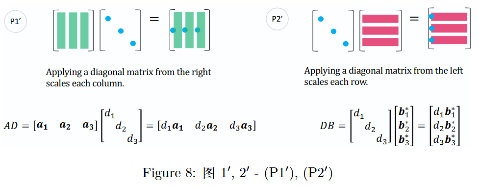
图 8:图 1′,2′ -(P 1 ′ P1'P1′),(P 2 ′ P2'P2′)
Applying Diagonal Matrices
对角矩阵的应用(P 1 ′ P1'P1′)是将对角矩阵D DD的对角线上的数分别乘以矩阵X XX的列向量,即X D XDXD 的第 j jj 列是 d j x j d_j x_jdjxj;
Applying a diagonal matrix from the right scales each column.
从右侧应用对角矩阵会缩放每一列。(P 2 ′ P2'P2′)是将对角矩阵D DD的对角线上的数分别乘以矩阵X XX的行向量,即D X DXDX 的第 i ii 行是 d i x i ∗ d_i x_i^*dixi∗。
Applying a diagonal matrix from the left scales each row.
从左侧应用对角矩阵会缩放每一行。
(就是二者分别P 1 P1P1)和(P 2 P2P2)的变体。
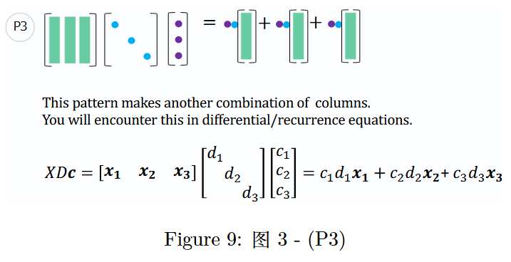
图 9:图 3 -(P 3 P3P3)
Column Combinations in Differential/Recurrence Equations
微分/递归方程中的列组合This pattern makes another combination of columns. You will encounter this in differential/recurrence equations.
这种模式构成了另一组列的组合。你将在微分/递归方程中遇到这种情况。X D C = [ x 1 x 2 x 3 ] [ d 1 d 2 d 3 ] [ c 1 c 2 c 3 ] = c 1 d 1 x 1 + c 2 d 2 x 2 + c 3 d 3 x 3 XDC=\begin{bmatrix}x_1&x_2&x_3\end{bmatrix}\begin{bmatrix}d_1&&\\&d_2&\\&&d_3\end{bmatrix}\begin{bmatrix}c_1\\c_2\\c_3\end{bmatrix}=c_1d_1x_1 + c_2d_2x_2 + c_3d_3x_3XDC=[x1x2x3]d1d2d3c1c2c3=c1d1x1+c2d2x2+c3d3x3
该模式在求解微分方程和递归方程时也会出现:6 节(p. 201)特征值与特征向量(Eigenvalues and Eigenvectors)
6.4 节(p. 243)微分方程组(Systems of Differential Equations)
解微分方程和差分方程
考虑以下微分方程和差分方程:
微分方程
d u ( t ) d t = A u ( t ) , u ( 0 ) = u 0 \frac{du(t)}{dt} = Au(t), \quad u(0) = u_0dtdu(t)=Au(t),u(0)=u0差分方程
u n + 1 = A u n , u 0 = u 0 u_{n+1} = Au_n, \quad u_0 = u_0un+1=Aun,u0=u0初始值的表示
u 0 = c 1 x 1 + c 2 x 2 + c 3 x 3 u_0 = c_1 x_1 + c_2 x_2 + c_3 x_3u0=c1x1+c2x2+c3x3系数向量 c cc行通过以下方式计算:
c = [ c 1 c 2 c 3 ] = X − 1 u 0 c = \begin{bmatrix} c_1 \\ c_2 \\ c_3 \end{bmatrix} = X^{-1} u_0c=c1c2c3=X−1u0通解
对于微分方程,通解为:
u ( t ) = e A t u 0 = X e Λ t X − 1 u 0 = X e Λ t c = c 1 e λ 1 t x 1 + c 2 e λ 2 t x 2 + c 3 e λ 3 t x 3 u(t) = e^{At}u_0 = Xe^{\Lambda t}X^{-1}u_0 = Xe^{\Lambda t}c = c_1 e^{\lambda_1 t} x_1 + c_2 e^{\lambda_2 t} x_2 + c_3 e^{\lambda_3 t} x_3u(t)=eAtu0=XeΛtX−1u0=XeΛtc=c1eλ1tx1+c2eλ2tx2+c3eλ3tx3对于差分方程,通解为:
u n = A n u 0 = X Λ n X − 1 u 0 = X Λ n c = c 1 λ 1 n x 1 + c 2 λ 2 n x 2 + c 3 λ 3 n x 3 u_n = A^n u_0 = X \Lambda^n X^{-1} u_0 = X \Lambda^n c = c_1 \lambda_1^n x_1 + c_2 \lambda_2^n x_2 + c_3 \lambda_3^n x_3un=Anu0=XΛnX−1u0=XΛnc=c1λ1nx1+c2λ2nx2+c3λ3nx3见图 9:通过步骤 P3 可以得到X D c XDcXDc。
对于这两种疑问,它们的解都可以用矩阵A AA 的特征值 ( λ 1 , λ 2 , λ 3 ) (\lambda_1, \lambda_2, \lambda_3)(λ1,λ2,λ3)、特征向量 X = [ x 1 x 2 x 3 ] X = [x_1 \ x_2 \ x_3]X=[x1x2x3] 和系数向量 c = [ c 1 c 2 c 3 ] T c = \begin{bmatrix} c_1 & c_2 & c_3 \end{bmatrix}^Tc=[c1c2c3]T来表示。其中,c cc 是以 X XX为基底的初始值u ( 0 ) = u 0 u(0) = u_0u(0)=u0 的坐标。
以上两个问题的通解基于初始条件u 0 = c 1 x 1 + c 2 x 2 + c 3 x 3 u_0 = c_1x_1 + c_2x_2 + c_3x_3u0=c1x1+c2x2+c3x3,通过 P 3 P3P3模式可推导出后续的解表达式。
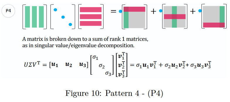
图 10:模式 4 -(P 4 P_4P4)
P 4 P_4P4在特征值分解和奇异值分解中都会用到。这两种分解都可以表示为三个矩阵的乘积,且中间的矩阵均为对角矩阵,同时也都能表示为带有特征值/奇异值系数的秩 1 矩阵之和。更多细节将在下一节中展开讨论。
Singular Value/Eigenvalue Decomposition
奇异值/特征值分解A matrix is broken down to a sum of rank 1 matrices, as in singular value/eigenvalue decomposition.
矩阵被分解为秩为 1 的矩阵之和,如奇异值/特征值分解。U Σ V T = [ u 1 u 2 u 3 ] [ σ 1 σ 2 σ 3 ] [ v 1 T v 2 T v 3 T ] = σ 1 u 1 v 1 T + σ 2 u 2 v 2 T + σ 3 u 3 v 3 T U \Sigma V^T = [u_1 \quad u_2 \quad u_3] \begin{bmatrix} \sigma_1 & & \\ & \sigma_2 & \\ & & \sigma_3 \end{bmatrix} \begin{bmatrix} v_1^T \\ v_2^T \\ v_3^T \end{bmatrix} = \sigma_1 u_1 v_1^T + \sigma_2 u_2 v_2^T + \sigma_3 u_3 v_3^TUΣVT=[u1u2u3]σ1σ2σ3v1Tv2Tv3T=σ1u1v1T+σ2u2v2T+σ3u3v3T
其中 U UU 和 V VV是正交矩阵,Σ \SigmaΣ是包含奇异值σ 1 , σ 2 , σ 3 \sigma_1, \sigma_2, \sigma_3σ1,σ2,σ3的对角矩阵。原始矩阵被表示为秩 1 矩阵之和,每个矩阵都乘以其对应的奇异值。
一种将原始矩阵就是奇异值分解A AA分解为一系列更简单矩阵乘积的办法。
原始矩阵 A AA可以通过这三个矩阵的乘积来重构:
A = U Σ V T A = U \Sigma V^TA=UΣVT
这种分解不仅适用于方阵,也适用于非方阵。分解的结果由三个部分组成:
U UU(左奇异向量矩阵): m × m m \times mm×m的正交矩阵,其列向量称为左奇异向量。这些向量是原始矩阵A AA的行空间的正交基。
Σ \SigmaΣ(奇异值对角矩阵): m × n m \times nm×n的对角矩阵,对角线上的元素是非负的奇异值,通常按从大到小的顺序排列。奇异值表示原始矩阵A AA在对应奇异向量方向上的“拉伸”或“压缩”程度。
V T V^TVT(右奇异向量矩阵的转置): n × n n \times nn×n的正交矩阵,其行向量称为右奇异向量。这些向量是原始矩阵A AA的列空间的正交基。
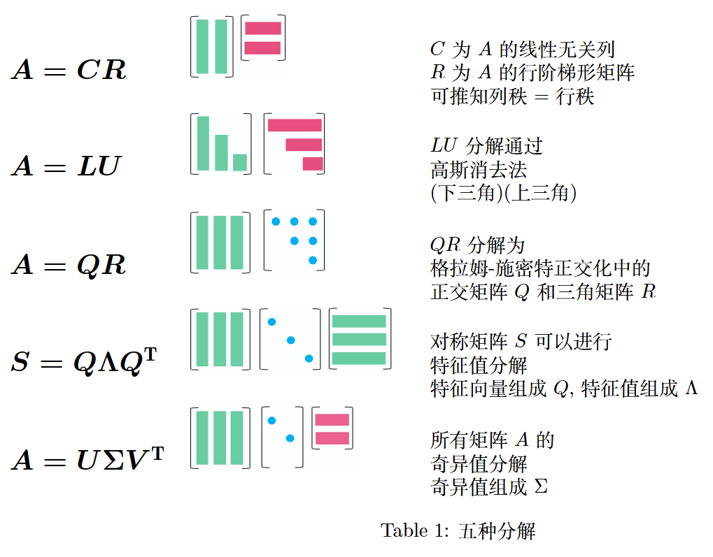
6 矩阵的 5 种分解
- 前言第 vii 页,本书大纲(The Plan for the Book):将依次对A = C R A = CRA=CR(列 - 行分解)、A = L U A = LUA=LU(高斯消去分解)、A = Q R A = QRA=QR(正交三角分解)、S = Q Λ Q T S = Q\Lambda Q^TS=QΛQT(对称矩阵特征值分解)、A = U Σ V T A = U\Sigma V^TA=UΣVT(奇异值分解)进行说明。
分解类型说明
| 分解类型 | 说明 |
|---|---|
| A = C R A = CRA=CR(列-行分解) | C CC 为矩阵 A AA的线性无关列向量构成的矩阵,R RR 为矩阵 A AA的行阶梯形矩阵(消除零行),可由此推知列秩 = 行秩 |
| A = L U A = LUA=LU(高斯消去分解) | 通过高斯消去法将矩阵A AA分解为下三角矩阵L LL(Lower Triangular Matrix)和上三角矩阵U UU(Upper Triangular Matrix)的乘积 |
| A = Q R A = QRA=QR(正交三角分解) | 基于格拉姆-施密特正交化,将矩阵A AA分解为正交矩阵Q QQ(Orthogonal Matrix)和上三角矩阵R RR(Upper Triangular Matrix)的乘积 |
| S = Q Λ Q T S = Q\Lambda Q^TS=QΛQT(对称矩阵特征值分解) | 对称矩阵 S SS(S = S T S = S^TS=ST)可分解为正交矩阵Q QQ(由特征向量构成)、对角矩阵Λ \LambdaΛ(由特征值构成)与Q QQ 的转置矩阵 Q T Q^TQT 的乘积 |
| A = U Σ V T A = U\Sigma V^TA=UΣVT(奇异值分解) | 所有矩阵 A AA都可进行奇异值分解,其中U UU(左奇异向量构成)和V VV(右奇异向量构成)为正交矩阵,Σ \SigmaΣ(由奇异值构成)为对角矩阵 |
6.1 A = C R A = CRA=CR(列 - 行分解)
1.4 节 矩阵乘法与A = C R A = CRA=CR分解(Matrix Multiplication andA = C R A = CRA=CR)(p. 29)
所有一般的长矩阵A AA(m × n m\times nm×n 矩阵,m ≠ n m\neq nm=n)都具有相同的行秩和列秩,A = C R A = CRA=CR理解这一定理最直观的方法。其中,就是分解C CC 由 A AA的线性无关列向量构成,R RR 为 A AA的行阶梯形矩阵(已消除零行)。该分解本质是将矩阵A AA化简为其线性无关列向量构成的矩阵C CC和线性无关行向量构成的矩阵R RR 的乘积。
A = C R [ 1 2 3 2 3 5 ] = [ 1 2 2 3 ] [ 1 0 1 0 1 1 ] \begin{aligned} A &= CR \\ \\ \begin{bmatrix} 1 & 2 & 3 \\ 2 & 3 & 5 \end{bmatrix} &= \begin{bmatrix} 1 & 2 \\ 2 & 3 \end{bmatrix} \begin{bmatrix} 1 & 0 & 1 \\ 0 & 1 & 1 \end{bmatrix} \end{aligned}A[122335]=CR=[1223][100111]
推导过程:从左至右观察矩阵A AA的列向量,保留其中线性无关的列向量,去掉可由前面保留的列向量线性表出的列向量。例如,若矩阵A AA的第 1、2 列线性无关,第 3 列可由前两列之和表示,则保留第 1、2 列构成C CC;若要通过 C CC 重新构造出 A AA,则需要右乘一个行阶梯矩阵R RR。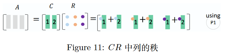
图 11:矩阵 A AA 中列的秩
此时可发现,矩阵A AA的列秩为 2,因为C CC中仅包含 2 个线性无关的列向量,且A AA中所有的列向量都可由C CC中的这 2 个列向量线性表出。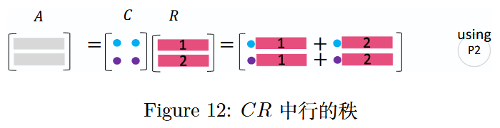
图 12:矩阵 A AA 中行的秩
同理,矩阵 A AA的行秩也为 2,因为R RR中仅包含 2 个线性无关的行向量,且A AA中所有的行向量都可由R RR中的这 2 个行向量线性表出。
6.2 A = L U A = LUA=LU(高斯消去分解)
用高斯消除法求解线性方程组A x = b Ax = bAx=b的过程,本质上就是对矩阵A AA 进行 L U LULU分解。通常,L U LULU分解是通过对矩阵A AA左乘一系列初等行变换矩阵E EE,将其转化为上三角矩阵U UU,即 E A = U EA = UEA=U,进而可得 A = E − 1 U A = E^{-1}UA=E−1U,令 L = E − 1 L = E^{-1}L=E−1(L LL为下三角矩阵),则A = L U A = LUA=LU。
E A = U A = E − 1 U let L = E − 1 , A = L U \begin{align*} EA &= U \\ A &= E^{-1}U \\ \text{let } L = E^{-1}, \quad A &= LU \end{align*}EAAlet L=E−1,A=U=E−1U=LU
现在, 求解A x = b Ax = bAx=b有 2 步: (1) 求解L c = b Lc = bLc=b, (2) 代回U x = c Ux = cUx=c.
- 2.3 节(p. 57)矩阵计算与A = L U A = LUA=LU分解(Matrix Computations andA = L U A = LUA=LU)
在这里,我们直接通过A AA 计算 L LL 和 U UU: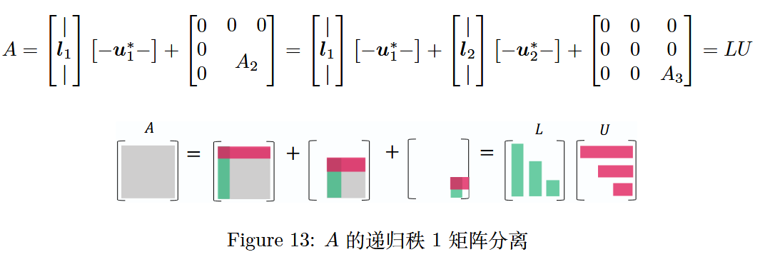
图 13:矩阵 A AA的递归秩 1 矩阵分离
要计算 L LL 和 U UU,首先分离出由矩阵A AA 的第一行 u 1 ∗ u_1^*u1∗ 和第一列 l 1 l_1l1 组成的外积 l 1 u 1 ∗ l_1 u_1^*l1u1∗,余下的部分记为A 2 A_2A2;然后对 A 2 A_2A2递归执行此操作,最终将矩阵A AA分解为若干个秩 1 矩阵之和,进而得到L LL 和 U UU。
分离:
每次只拆分当前矩阵的“首列首行”,留下右下角剩余子块。递归
用同一分离规则拆分剩余部分,重复操作直到剩余子块为零。步骤
第 1 次分离:由A AA的“首列分块l 1 \boldsymbol{l}_1l1”和“首行分块u 1 ∗ \boldsymbol{u}_1^*u1∗”相乘得到的“秩 1 分块矩阵”(l 1 u 1 ∗ \boldsymbol{l}_1 \boldsymbol{u}_1^*l1u1∗);
A → l 1 u 1 ∗ + A 2 A \to \boldsymbol{l}_1 \boldsymbol{u}_1^* + A_2A→l1u1∗+A2;第 2 次分离:不再处理第一步已拆分的l 1 u 1 ∗ \boldsymbol{l}_1 \boldsymbol{u}_1^*l1u1∗,而是针对除l 1 u 1 ∗ \boldsymbol{l}_1 \boldsymbol{u}_1^*l1u1∗的“右下角子块A 2 A_2A2”,再次进行“分离”——将A 2 A_2A2 拆成l 2 u 2 ∗ \boldsymbol{l}_2 \boldsymbol{u}_2^*l2u2∗,以及新的子块A 3 A_3A3。
A 2 → l 2 u 2 ∗ + A 3 A_2 \to \boldsymbol{l}_2 \boldsymbol{u}_2^* + A_3A2→l2u2∗+A3,代入第一步得A → l 1 u 1 ∗ + l 2 u 2 ∗ + A 3 A \to \boldsymbol{l}_1 \boldsymbol{u}_1^* + \boldsymbol{l}_2 \boldsymbol{u}_2^* + A_3A→l1u1∗+l2u2∗+A3;
……
直到第 r rr次分离:剩余子块为零矩阵(即A k + 1 = 0 A_{k+1} = 0Ak+1=0),当剩余子块不再包含有效信息(秩为 0)时,停止拆分,此时所有非零信息已被完全分解到l k u k ∗ \boldsymbol{l}_k \boldsymbol{u}_k^*lkuk∗ 项中,得到 r rr个非零分块项l 1 u 1 ∗ , l 2 u 2 ∗ , … , l r u r ∗ \boldsymbol{l}_1 \boldsymbol{u}_1^*, \boldsymbol{l}_2 \boldsymbol{u}_2^*, \dots, \boldsymbol{l}_r \boldsymbol{u}_r^*l1u1∗,l2u2∗,…,lrur∗,且 r rr 正是矩阵 A AA的秩(非零子块的最大数量)。最终分解式为:
A = ∑ k = 1 r l k u k ∗ = L U A = \sum_{k=1}^r \boldsymbol{l}_k \boldsymbol{u}_k^* = LUA=∑k=1rlkuk∗=LU(L LL 由 l 1 , l 2 , … , l r \boldsymbol{l}_1,\boldsymbol{l}_2,…,\boldsymbol{l}_rl1,l2,…,lr 组成,U UU 由 u 1 ∗ , u 2 ∗ , … , u r ∗ \boldsymbol{u}_1^*,\boldsymbol{u}_2^*,…,\boldsymbol{u}_r^*u1∗,u2∗,…,ur∗ 组成)。
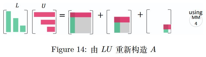
图 14:由 L U LULU重新构造矩阵A AA
通过下三角矩阵L LL乘以上三角矩阵U UU来重新构造矩阵A AA相对简单,即A = L U A = LUA=LU。
6.3 A = Q R A = QRA=QR(正交三角分解)
QR 分解是在保持矩阵A AA列空间不变(即C ( A ) = C ( Q ) C(A) = C(Q)C(A)=C(Q))的条件下,将矩阵A AA 表示为 列正交矩阵 Q QQ 与 上三角矩阵 R RR 的乘积,即 A = Q R A = QRA=QR。
其中,Q QQ的列向量是通过对A AA的列向量组进行正交化与单位化得到的标准正交向量组,它们构成A AA列空间的一组标准正交基。若A AA是可逆方阵,则Q QQ为正交矩阵(满足Q Q T = Q T Q = I QQ^T = Q^TQ = IQQT=QTQ=I)。
- 4.4 节 正交矩阵与格拉姆 - 施密特正交化(Orthogonal matrices and Gram - Schmidt)(p. 165)
以 3 维列向量为例,格拉姆 - 施密特正交化通过以下步骤构造正交矩阵Q QQ 的列向量:
第一个列向量的单位化
对 A AA的第一个列向量a 1 \boldsymbol{a}_1a1,单位化后得到q 1 \boldsymbol{q}_1q1:
q 1 = a 1 ∥ a 1 ∥ \boldsymbol{q}_1 = \frac{\boldsymbol{a}_1}{\|\boldsymbol{a}_1\|}q1=∥a1∥a1
其中 ∥ a 1 ∥ \|\boldsymbol{a}_1\|∥a1∥ 是 a 1 \boldsymbol{a}_1a1的欧几里得范数,即∥ a 1 ∥ = a 1 T a 1 \|\boldsymbol{a}_1\| = \sqrt{\boldsymbol{a}_1^T \boldsymbol{a}_1}∥a1∥=a1Ta1。第二个列向量的正交化与单位化
对 A AA的第二个列向量a 2 \boldsymbol{a}_2a2,先减去其在q 1 \boldsymbol{q}_1q1上的投影,得到与q 1 \boldsymbol{q}_1q1正交的临时向量q 2 temp \boldsymbol{q}_2^{\text{temp}}q2temp;再对 q 2 temp \boldsymbol{q}_2^{\text{temp}}q2temp单位化,得到q 2 \boldsymbol{q}_2q2:
q 2 temp = a 2 − ( q 1 T a 2 ) q 1 , q 2 = q 2 temp ∥ q 2 temp ∥ \boldsymbol{q}_2^{\text{temp}} = \boldsymbol{a}_2 - (\boldsymbol{q}_1^T \boldsymbol{a}_2)\boldsymbol{q}_1, \quad \boldsymbol{q}_2 = \frac{\boldsymbol{q}_2^{\text{temp}}}{\|\boldsymbol{q}_2^{\text{temp}}\|}q2temp=a2−(q1Ta2)q1,q2=∥q2temp∥q2temp第三个列向量的正交化与单位化
对 A AA的第三个列向量a 3 \boldsymbol{a}_3a3,减去其在 q 1 \boldsymbol{q}_1q1 和 q 2 \boldsymbol{q}_2q2上的投影,得到与q 1 , q 2 \boldsymbol{q}_1, \boldsymbol{q}_2q1,q2正交的临时向量q 3 temp \boldsymbol{q}_3^{\text{temp}}q3temp;再对 q 3 temp \boldsymbol{q}_3^{\text{temp}}q3temp单位化,得到q 3 \boldsymbol{q}_3q3:
q 3 temp = a 3 − ( q 1 T a 3 ) q 1 − ( q 2 T a 3 ) q 2 , q 3 = q 3 temp ∥ q 3 temp ∥ \boldsymbol{q}_3^{\text{temp}} = \boldsymbol{a}_3 - (\boldsymbol{q}_1^T \boldsymbol{a}_3)\boldsymbol{q}_1 - (\boldsymbol{q}_2^T \boldsymbol{a}_3)\boldsymbol{q}_2, \quad \boldsymbol{q}_3 = \frac{\boldsymbol{q}_3^{\text{temp}}}{\|\boldsymbol{q}_3^{\text{temp}}\|}q3temp=a3−(q1Ta3)q1−(q2Ta3)q2,q3=∥q3temp∥q3temp
从列向量表示推导A = Q R A = QRA=QR
记 r i j = q i T a j r_{ij} = \boldsymbol{q}_i^T \boldsymbol{a}_jrij=qiTaj(i , j = 1 , 2 , 3 i,j = 1,2,3i,j=1,2,3),则矩阵 A AA的列向量可由Q QQ的列向量线性表出:
第一个列向量:a 1 = r 11 q 1 \boldsymbol{a}_1 = r_{11}\boldsymbol{q}_1a1=r11q1;
第二个列向量:a 2 = r 12 q 1 + r 22 q 2 \boldsymbol{a}_2 = r_{12}\boldsymbol{q}_1 + r_{22}\boldsymbol{q}_2a2=r12q1+r22q2;
第三个列向量:a 3 = r 13 q 1 + r 23 q 2 + r 33 q 3 \boldsymbol{a}_3 = r_{13}\boldsymbol{q}_1 + r_{23}\boldsymbol{q}_2 + r_{33}\boldsymbol{q}_3a3=r13q1+r23q2+r33q3。
将这些线性关系以矩阵形式整合,可得A = Q R A = QRA=QR。其中:
- Q = [ q 1 q 2 q 3 ] Q = \begin{bmatrix} \boldsymbol{q}_1 & \boldsymbol{q}_2 & \boldsymbol{q}_3 \end{bmatrix}Q=[q1q2q3]为正交矩阵(满足Q Q T = Q T Q = I QQ^T = Q^TQ = IQQT=QTQ=I);
- R RR为上三角矩阵,形式为:
R = [ r 11 r 12 r 13 r 22 r 23 r 33 ] R = \begin{bmatrix} r_{11} & r_{12} & r_{13} \\ & r_{22} & r_{23} \\ & & r_{33} \end{bmatrix}R=r11r12r22r13r23r33
因此,原矩阵A AA最终表示为“正交矩阵Q QQ与上三角矩阵R RR的乘积”,即:
A = Q R = [ ∣ ∣ ∣ q 1 q 2 q 3 ∣ ∣ ∣ ] [ r 11 r 12 r 13 r 22 r 23 r 33 ] A = QR = \begin{bmatrix} \mid & \mid & \mid \\ \boldsymbol{q}_1 & \boldsymbol{q}_2 & \boldsymbol{q}_3 \\ \mid & \mid & \mid \end{bmatrix} \begin{bmatrix} r_{11} & r_{12} & r_{13} \\ & r_{22} & r_{23} \\ & & r_{33} \end{bmatrix}A=QR=∣q1∣∣q2∣∣q3∣r11r12r22r13r23r33
其中 R RR的元素满足:r i j = q i T a j r_{ij} = \boldsymbol{q}_i^T \boldsymbol{a}_jrij=qiTaj(i ≤ j i \leq ji≤j),r i j = 0 r_{ij} = 0rij=0(i > j i > ji>j)。
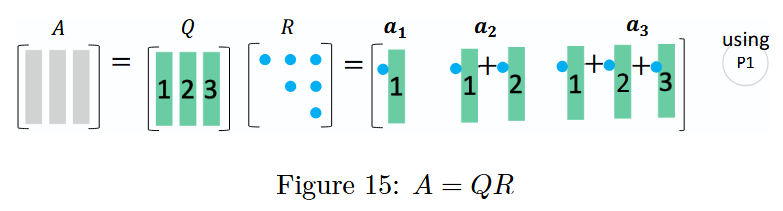
图 15:A = Q R A = QRA=QR 分解
通过 Q R QRQR 分解,矩阵 A AA的列向量被转化为正交矩阵Q QQ的列向量(一个正交集合),且矩阵A AA的每一个列向量都可以用Q QQ和上三角矩阵R RR重新构造出来,具体可参考前面的P 1 P1P1模式(列运算)。
6.4 S = Q Λ Q T S = Q\Lambda Q^TS=QΛQT(对称矩阵特征值分解)
所有对称矩阵S SS(满足 S = S T S = S^TS=ST)都具有实特征值和正交的特征向量。其中,特征值λ i \lambda_iλi 是对角矩阵 Λ \LambdaΛ的对角元素,特征向量q i q_iqi构成正交矩阵Q QQ 的列向量。
6.3 节(p. 227)对称正定矩阵(Symmetric Positive Definite Matrices)
对称矩阵 S SS的特征值分解表达式为:
S = Q Λ Q T = [ ∣ ∣ ∣ q 1 q 2 q 3 ∣ ∣ ∣ ] [ λ 1 λ 2 λ 3 ] [ − q 1 T − − q 2 T − − q 3 T − ] S=Q\Lambda Q^T=\begin{bmatrix}\mid&\mid&\mid\\q_1&q_2&q_3\\\mid&\mid&\mid\end{bmatrix}\begin{bmatrix}\lambda_1&&\\&\lambda_2&\\&&\lambda_3\end{bmatrix}\begin{bmatrix}-q_1^T -\\-q_2^T -\\-q_3^T -\end{bmatrix}S=QΛQT=∣q1∣∣q2∣∣q3∣λ1λ2λ3−q1T−−q2T−−q3T−进一步展开为秩 1 投影矩阵的线性组合:
S = λ 1 [ ∣ q 1 ∣ ] [ − q 1 T − ] + λ 2 [ ∣ q 2 ∣ ] [ − q 2 T − ] + λ 3 [ ∣ q 3 ∣ ] [ − q 3 T − ] = λ 1 P 1 + λ 2 P 2 + λ 3 P 3 \begin{aligned} S &= \lambda_1\begin{bmatrix}\mid\\q_1\\\mid\end{bmatrix}\begin{bmatrix}-q_1^T -\end{bmatrix} + \lambda_2\begin{bmatrix}\mid\\q_2\\\mid\end{bmatrix}\begin{bmatrix}-q_2^T -\end{bmatrix} + \lambda_3\begin{bmatrix}\mid\\q_3\\\mid\end{bmatrix}\begin{bmatrix}-q_3^T -\end{bmatrix} \\ &= \lambda_1 P_1 + \lambda_2 P_2 + \lambda_3 P_3 \end{aligned}S=λ1∣q1∣[−q1T−]+λ2∣q2∣[−q2T−]+λ3∣q3∣[−q3T−]=λ1P1+λ2P2+λ3P3
P 1 = q 1 q 1 T , P 2 = q 2 q 2 T , P 3 = q 3 q 3 T P_1 = q_1 q_1^{\text{T}}, \quad P_2 = q_2 q_2^{\text{T}}, \quad P_3 = q_3 q_3^{\text{T}}P1=q1q1T,P2=q2q2T,P3=q3q3T
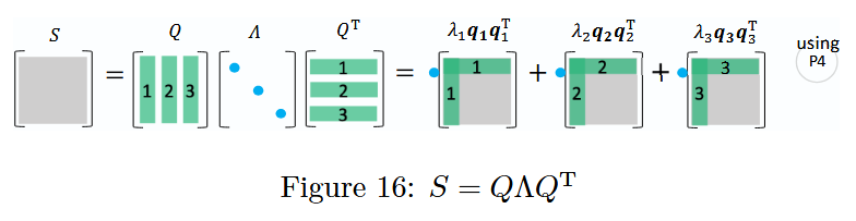
图 16:对称矩阵特征值分解
对称矩阵的谱定理
一个对称矩阵S SS可通过正交矩阵Q QQ及其转置矩阵Q T Q^TQT对角化为对角矩阵Λ \LambdaΛ,并且能进一步分解为一阶投影矩阵P i = q i q i T P_i = \boldsymbol{q}_i \boldsymbol{q}_i^TPi=qiqiT(其中 q i \boldsymbol{q}_iqi 是 Q QQ的列向量)的线性组合,这一结论即为谱定理(Spectral Theorem)。
分解的性质
此处的分解依赖于特定的性质(记为P 4 P_4P4),相关关系与投影矩阵P i P_iPi的性质如下:
对称矩阵的组合表示:
对称矩阵 S SS(满足 S = S T S = S^TS=ST)可表示为特征值与对应投影矩阵的线性组合:
S = S T = λ 1 P 1 + λ 2 P 2 + λ 3 P 3 S = S^T = \lambda_1 P_1 + \lambda_2 P_2 + \lambda_3 P_3S=ST=λ1P1+λ2P2+λ3P3
其中 λ 1 , λ 2 , λ 3 \lambda_1, \lambda_2, \lambda_3λ1,λ2,λ3 是 S SS 的特征值,P 1 , P 2 , P 3 P_1, P_2, P_3P1,P2,P3是对应一阶投影矩阵。单位矩阵的分解:
正交矩阵 Q QQ满足列向量的“完备性”,即各投影矩阵之和为单位矩阵I II:
Q Q T = P 1 + P 2 + P 3 = I Q Q^T = P_1 + P_2 + P_3 = IQQT=P1+P2+P3=I投影矩阵的自身性质:
- 对称性与幂等性:P i 2 = P i = P i T P_i^2 = P_i = P_i^TPi2=Pi=PiT(投影矩阵自身平方等于自身,且转置等于自身);
- 正交性:当 i ≠ j i \neq ji=j 时,P i P j = O P_i P_j = OPiPj=O(不同投影矩阵的乘积为零矩阵O OO)。
6.5 A = U Σ V T A = U\Sigma V^TA=UΣVT(奇异值分解)
- 7.1 节(p. 259)奇异值与奇异向量(Singular Values and Singular Vectors)
包括长方阵(m ≠ n m\neq nm=n)在内的所有矩阵都具有奇异值分解(SVD)。在A = U Σ V T A = U\Sigma V^TA=UΣVT 中,U UU(m × m m\times mm×m矩阵)的列向量是A A T AA^TAAT的特征向量(称为左奇异向量),V VV(n × n n\times nn×n矩阵)的列向量是A T A A^T AATA的特征向量(称为右奇异向量),Σ \SigmaΣ(m × n m\times nm×n矩阵)的对角线上的元素是A T A A^T AATA(或 A A T AA^TAAT)非零特征值的平方根(称为奇异值),非对角线元素均为 0。
简化版 SVD 特点:
- 正交性:U U T = I m U U^T = I_mUUT=Im(I m I_mIm 为 m mm阶单位矩阵),V V T = I n V V^T = I_nVVT=In(I n I_nIn 为 n nn阶单位矩阵),即U UU 和 V VV均为正交矩阵。
- 对角化作用:U T A V = Σ U^T A V = \SigmaUTAV=Σ,即通过 U T U^TUT(左乘)和 V VV(右乘)将矩阵A AA 对角化为 Σ \SigmaΣ。
- 秩 1 组合形式:A = U Σ V T = ∑ k = 1 r σ k u k v k T A = U\Sigma V^T=\sum_{k = 1}^r \sigma_k u_k v_k^TA=UΣVT=∑k=1rσkukvkT,其中 r rr 为矩阵 A AA 的秩,σ k \sigma_kσk 为奇异值,u k u_kuk为左奇异向量,v k v_kvk为右奇异向量,该式将A AA表示为秩 1 矩阵的线性组合。
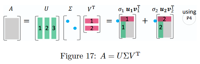
图 17:矩阵分解(SVD)A = U Σ V T A = U\Sigma V^TA=UΣVT
奇异值分解是通过正交矩阵U UU 和 V VV以及对角矩阵Σ \SigmaΣ,将任意矩阵A AA分解为具有明确几何意义(如旋转、缩放、投影)的矩阵乘积形式。
可以发现:
- V VV 是 R n \mathbb{R}^nRn 空间中 A T A A^T AATA的特征向量构成的标准正交基;
- U UU 是 R m \mathbb{R}^mRm 空间中 A A T A A^TAAT的特征向量构成的标准正交基。
U UU 和 V VV 共同将矩阵 A AA对角化为对角矩阵Σ \SigmaΣ,且 A AA 还可表示为秩 1 矩阵的线性组合,具体推导如下:
A = U Σ V T = [ ∣ ∣ ∣ u 1 u 2 u 3 ∣ ∣ ∣ ] [ σ 1 σ 2 ] [ − v 1 T − − v 2 T − ] = σ 1 [ ∣ u 1 ∣ ] [ − v 1 T − ] + σ 2 [ ∣ u 2 ∣ ] [ − v 2 T − ] = σ 1 u 1 v 1 T + σ 2 u 2 v 2 T \begin{align*} A &= U\Sigma V^T \\ &= \begin{bmatrix} \mid & \mid & \mid \\ \boldsymbol{u}_1 & \boldsymbol{u}_2 & \boldsymbol{u}_3 \\ \mid & \mid & \mid \end{bmatrix} \begin{bmatrix} \sigma_1 & \\ & \sigma_2 \\ & \end{bmatrix} \begin{bmatrix} - \boldsymbol{v}_1^T - \\ - \boldsymbol{v}_2^T - \end{bmatrix} \\ &= \sigma_1 \begin{bmatrix} \mid \\ \boldsymbol{u}_1 \\ \mid \end{bmatrix} \begin{bmatrix} - \boldsymbol{v}_1^T - \end{bmatrix} + \sigma_2 \begin{bmatrix} \mid \\ \boldsymbol{u}_2 \\ \mid \end{bmatrix} \begin{bmatrix} - \boldsymbol{v}_2^T - \end{bmatrix} \\ &= \sigma_1 \boldsymbol{u}_1 \boldsymbol{v}_1^T + \sigma_2 \boldsymbol{u}_2 \boldsymbol{v}_2^T \end{align*}A=UΣVT=∣u1∣∣u2∣∣u3∣σ1σ2[−v1T−−v2T−]=σ1∣u1∣[−v1T−]+σ2∣u2∣[−v2T−]=σ1u1v1T+σ2u2v2T
注意
正交矩阵 U UU 和 V VV 满足:
- U U T = I m U U^T = I_mUUT=Im(I m I_mIm 为 m × m m \times mm×m 单位矩阵)
- V V T = I n V V^T = I_nVVT=In(I n I_nIn 为 n × n n \times nn×n 单位矩阵)
奇异值分解的图释细节可参考P 4 P_4P4。
总结和致谢
我展示了矩阵/向量乘法的系统可视化表达,以及这些表达在五种矩阵分解中的应用。希望大家能喜欢这些内容,并经过它们加深对线性代数的理解。
阿什利·费尔南德斯(Ashley Fernandes)在排版过程中支援我美化了这篇论文,使其格式更统一、更专业。
在完成这篇论文之际,我要感谢吉尔伯特·斯特朗(Gilbert Strang)教授出版《人人都懂线性代数》(“Linear Algebra for Everyone”)一书。它引导大家从新的视角探索线性代数中的美妙内容,其中既介绍了当代与传统的数据科学和机器学习相关知识,也让每个人都能依据实用的方式理解线性代数的核心思想——这些都是矩阵世界的重要组成部分。
参考文献与相关工作
Gilbert Strang (2020), Linear Algebra for Everyone, Wellesley Cambridge Press.
Gilbert Strang (2016), Introduction to Linear Algebra, Wellesley Cambridge Press, 5th ed.
Kenji Hiranabe (2021), Map of Eigenvalues, An Agile Way (blog)
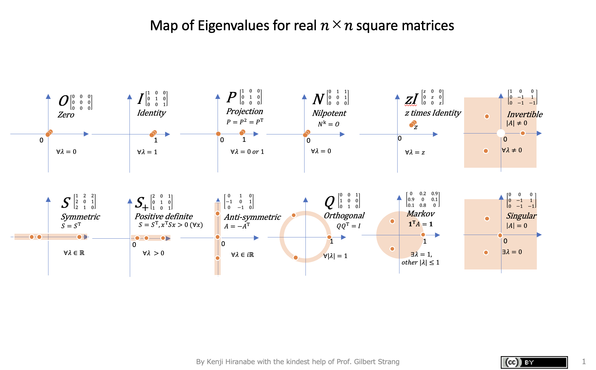
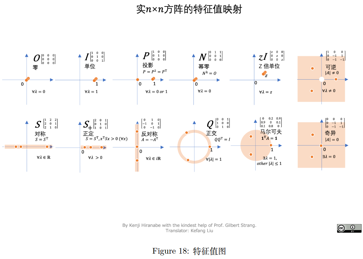
图 18:特征值图(实n × n n\times nn×n方阵的特征值映射)
Kenji Hiranabe (2020), Matrix World, An Agile Way (blog)
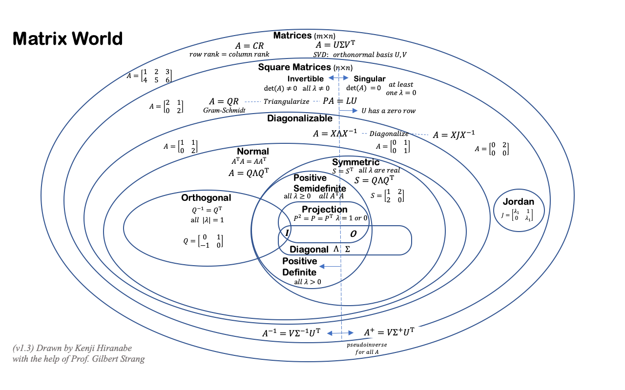
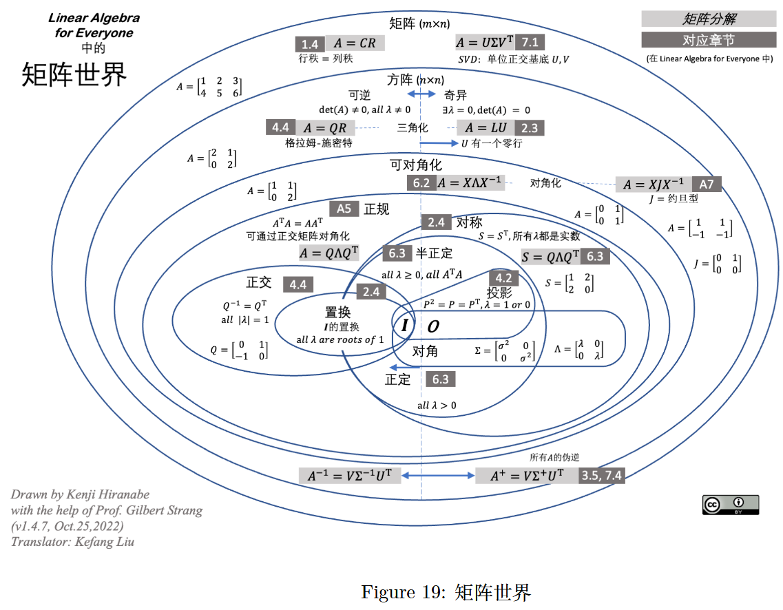
图 19:矩阵世界(Linear Algebra Matrix World)
(由 Kenji Hiranabe 在 Gilbert Strang 教授的帮助下绘制,版本 v1.4.7,2022 年 10 月 25 日,译者:刘克芳)New Ideas in “Linear Algebra for Everyone” Gilbert Strangi - compareLAFE-ILA5I
updated February 4, 2024
Essence of linear algebra
线性代数的本质
A geometric understanding of matrices, determinants, eigen-stuffs and more.
矩阵、行列式、特征值与特征向量等概念的几何视角解读
Vectors
向量
Always think vectors in the coordinate space
始终在坐标空间中理解向量It’s a directed line, starting at the origin, with certain length
向量是从原点出发、具有特定长度的有向线段Addition of vectors
向量的加法each vector represents a “movement” with steps and direction
每个向量都代表一次包含步长和方向的“移动”a sum of two vectors can be thought as a two-step movement: first step move with vector 1 and move 2 after the first step move
两个向量的和可理解为两次连续的移动:先沿第一个向量移动,再沿第二个向量移动Vector multiple by a number (“scalar”)
向量与数(“标量”)的乘法“stretching” each coordinate by the value of scalar
按标量的数值“拉伸”向量的每个坐标分量
Linear combinations, span, and basis vectors
线性组合、张成空间与基向量
- Span (of a vector): the line aligned with/goes through the vector
(单个向量的)张成空间:与该向量共线且经过该向量的直线
Linear transformation and matrices
线性变换与矩阵
“Linear” transformation (properties) => grid lines remain parallel and evenly spaced:
“线性”变换(性质):网格线保持平行且间距均匀,具体表现为:all lines remain as lines without getting curved
所有直线变换后仍为直线,不会弯曲the origin remain fixed
原点保持不动e.g. rotation, stretch
例如:旋转、拉伸It can be considered as where the base vectors (i ^ \hat{i}i^ and j ^ \hat{j}j^) land after transformation, then everything else (i.e. all the vectors) in the coordinate follows
线性变换可通过基向量(i ^ \hat{i}i^ 和 j ^ \hat{j}j^)变换后的落点来确定,坐标空间中的所有其他向量都会遵循基向量的变换规律if v → = c 1 i ^ + c 2 j ^ \text{if } \overrightarrow{v} = c_1 \hat{i} + c_2\hat{j}if v=c1i^+c2j^
and after transformation i ^ lands on i → and j ^ lands on j → \text{and after transformation } \hat{i} \text{ lands on } \overrightarrow{i} \text{ and } \hat{j} \text{ lands on }\overrightarrow{j}and after transformationi^lands oni and j^lands onj
且变换后 i ^ 落在 i → 处, j ^ 落在 j → 处 \text{且变换后 } \hat{i} \text{ 落在 } \overrightarrow{i} \text{ 处,}\hat{j} \text{ 落在 } \overrightarrow{j} \text{ 处}且变换后i^落在i处,j^落在j处then transformed v → can be written as v → ′ = c 1 i → + c 2 j → \text{then transformed } \overrightarrow{v} \text{ can be written as } \overrightarrow{v}' = c_1 \overrightarrow{i} + c_2\overrightarrow{j}then transformedvcan be written asv′=c1i+c2j
则变换后的 v → 可表示为 v → ′ = c 1 i → + c 2 j → \text{则变换后的 } \overrightarrow{v} \text{ 可表示为 } \overrightarrow{v}' = c_1 \overrightarrow{i} + c_2\overrightarrow{j}则变换后的v可表示为v′=c1i+c2jThus the linear transformation of a 2-dimensional vector can be fully described by a2 × 2 2 \times 22×2matrix defined by the vectorsi → \overrightarrow{i}i and j → \overrightarrow{j}j, or [ i → j → ] [\overrightarrow{i} \ \overrightarrow{j}][ij].
因此,二维向量的线性变换可由一个2 × 2 2 \times 22×2矩阵完整描述,该矩阵由变换后的基向量i → \overrightarrow{i}i 和 j → \overrightarrow{j}j 构成,即 [ i → j → ] [\overrightarrow{i} \ \overrightarrow{j}][ij]。Calculation of linear transformation of a vector as the dot product of a matrix with a vector:
向量的线性变换可通过矩阵与向量的点积计算,公式如下:
[ a b c d ] [ e f ] = e ∗ [ a c ] + f ∗ [ b d ] = [ a ∗ e + b ∗ f c ∗ e + d ∗ f ] \begin{split}\begin{bmatrix} a & b \\ c & d \end{bmatrix} \begin{bmatrix} e \\ f \end{bmatrix} = e * \begin{bmatrix} a\\ c \end{bmatrix} + f * \begin{bmatrix} b \\ d \end{bmatrix} = \begin{bmatrix} a*e + b*f \\ c*e + d*f \end{bmatrix}\end{split}[acbd][ef]=e∗[ac]+f∗[bd]=[a∗e+b∗fc∗e+d∗f]
Matrices multiplication can be thought as splitting the second matrix column-wise into individual column vectors, conduct above calculation for each column vector and combine the results column-wise.
矩阵乘法可理解为:将第二个矩阵按列拆分为单个列向量,对每个列向量分别执行上述矩阵与向量的乘法运算,最后将结果按列组合。Special linear transformation:
特殊的线性变换:Shear, whose transformation matrix is
剪切变换,其变换矩阵为
[ 1 1 0 1 ] \begin{split}\begin{bmatrix} 1 & 1 \\ 0 & 1\end{bmatrix} \end{split}[1011]
Linearly dependent transformation: the resulting transformed space is squashed into a 1-dimensional line
线性相关变换:变换后的空间被压缩成一条一维直线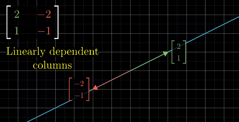
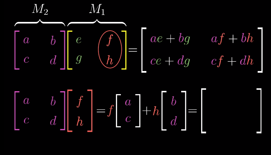
Matrix multiplication as composition
作为复合变换的矩阵乘法
Multiplication of two matrices ==> two-step transformation (composition) of the space geometrically
两个矩阵相乘,从几何角度看,等价于对空间进行两次连续的线性变换(即变换的复合)This is basically what I summarized in linear transformation:
这与前文线性变换部分的总结一致,如图所示:
This indicates that the order of the matrices multiplication matters, i.e. change the order of matrices will change the result
这表明矩阵乘法的顺序至关重要,即交换矩阵的相乘顺序会改变结果To compute the determinant
行列式的计算公式为
det ( [ a b c d ] ) = a d − b c \begin{split}\det\left(\begin{bmatrix} a & b \\ c & d\end{bmatrix} \right) = ad - bc\end{split}det([acbd])=ad−bc
Three-dimensional linear transformation
三维线性变换
Very similar to two-dimensional transformation
三维线性变换与二维线性变换相当相似Instead of move/transform thex − x-x− and y − y-y−coordinates, there is just an additionalz − z-z−axis to be transformed
区别在于:二维变换仅涉及x − x-x− 轴和 y − y-y−轴的变换,而三维变换还需额外考虑z − z-z− 轴的变换
The determinant
行列式
Geometric explanation: the “scaling” factor a linear transformation imposes to the area (2D) or volume (3D or above) defined by the basis vectors (since the area defined by the basis vectors is 1, the determinant is actually the signed area of the space defined by the column vectors in the transformation matrix)
线性变换对基向量所围成区域(二维中为面积,三维及以上为体积)的“缩放系数”。由于基向量围成的区域面积/体积为 1,因此行列式本质上等于变换矩阵列向量所围成空间的有向面积/体积。就是几何意义:行列式Determinant can be negative, depending on the orientation of the transformation (negative if orientation is inverted/flipped)
行列式可正可负,符号由变换的定向决定:若变换导致空间定向反转(翻转),则行列式为负。Determinant of zero meaning the transformation leads to 0 scaling to the area/volume or even to a single point; it also corresponds tolinearly dependent transformation
行列式为 0 意味着:变换将空间区域的面积/体积缩放至 0(甚至压缩成一个点),此种情况对应线性相关变换。Right-hand rule: to check the orientation of the transformation in 3D
右手定则:用于判断三维空间中变换的定向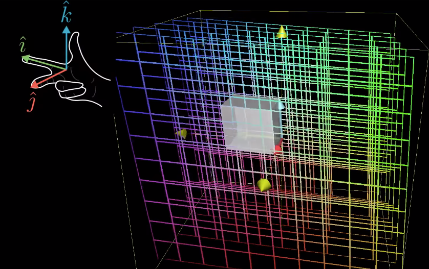
Inverse matrices, column space and null space
逆矩阵、列空间与零空间
Linear system of equations<=> matrix, vector product => linear transformation of a vector
线性方程组等价于 矩阵与向量的乘积,本质是向量的线性变换Inverse of a matrix=> a back transformation corresponds to the matrix itself
矩阵的逆是该矩阵所对应线性变换的“逆变换”(即撤销原变换的变换)The inverse of a matrix exists as long as its determinant is non-zero; in contrast, if the determinant is 0, the inverse doesn’t exist, i.e. we can expand a lower dimension space to a higher dimension one. There can be infinite possible higher dimensional space corresponds to the lower space in such case.
当且仅当矩阵的行列式非零时,其逆矩阵存在;反之,若行列式为 0,则逆矩阵不存在。这意味着:我们无法将低维空间“扩展”为高维空间,且一个低维空间可能对应无数个高维空间。In some special cases, when the determinant is 0, there may still be solutions to some vectors, when the output vectors are those lie along the lower dimension line/space after the transformation (why??)
在某些特殊情况下,即使行列式为 0,部分向量仍可能存在解:当输出向量恰好落在变换后低维直线/空间上时(原因待探究?)Rank:
秩:geometrically, it’s the number of dimensions of the resulting space/output after a linear transformation, e.g. if the transformation leads to a line, then the rank of the transformation matrix is 1;
几何意义:线性变换后输出空间的维数。例如,若变换将空间压缩成一条直线,则变换矩阵的秩为 1;Linear algebra: linearly independent columns of the transformation matrix
线性代数定义:变换矩阵中线性无关列向量的个数Column spaceof a matrix: set of all possible outputs of the linear transformation <=> the span of columns of the transformation matrix
矩阵的列空间:线性变换所有可能输出向量的集合,等价于变换矩阵列向量的张成空间Ranks of a matrix is the number of dimensions in its column space;[ 0 0 ] \begin{bmatrix}0\\0\end{bmatrix}[00]is always in the column space
矩阵的秩等于其列空间的维数,且零向量[ 0 0 ] \begin{bmatrix}0\\0\end{bmatrix}[00]始终在列空间中Full rank: when the rank is as high as it can be;
满秩:矩阵的秩达到其最大可能值;for a full rank transformation, only the original can lands on itself;
满秩变换中,只有零向量变换后仍为自身;for a non-full rank transformation, there are infinite numbers of vectors can land on the origin; it is a whole line of vectors in 2D cases or whole plane of vectors get squished into the origin in 3D cases (that the number of dimensions lost in the transformation).
非满秩变换中,有无数个向量变换后会落在原点:二维空间中是一整条直线上的向量,三维空间中是一整个平面上的向量(这些向量对应的维数即为变换中“丢失”的维数)。Null space: the set of vectors that lands on the origin or thekernelof the matrix
零空间(又称矩阵的核):变换后落在原点的所有向量的集合
Nonsquare matrices transformations between dimensions
非方阵:不同维度间的变换
Columns of the matrix stands for the number of basis vectors (in input)
矩阵的列数代表输入空间中基向量的个数(即输入空间的维数)Rows of the matrix stands for the number of coordinates of each landing spots (in output)
矩阵的行数代表输出空间中每个落点的坐标分量个数(即输出空间的维数)
Dot products and duality
点积与对偶性
Geometrical interpretation
几何意义Project one vector to the other vector, multiply the projected vector’s length with the length of the other vector
将一个向量投影到另一个向量上,再将投影向量的长度与被投影向量的长度相乘Numerical calculation
数值计算
[ a b ] ⋅ [ c d ] = [ a b ] ∗ [ c d ] = a ∗ c + b ∗ d \begin{split}\begin{bmatrix} a \\ b \end{bmatrix}\cdot \begin{bmatrix} c \\ d \end{bmatrix} = [a \ b] * \begin{bmatrix} c \\ d \end{bmatrix} = a*c + b*d\end{split}[ab]⋅[cd]=[ab]∗[cd]=a∗c+b∗d
- Connection between geometric interpretation and linear transformation of a vector
点积的几何意义与向量线性变换的关联
Dot product is equivalent to matrix-vector multiplication, i.e. a1 × 2 1\times 21×2matrix/vector times a2 × 1 2\times 12×1vector
点积等价于矩阵与向量的乘法,即一个1 × 2 1 \times 21×2矩阵(或行向量)与一个2 × 1 2 \times 12×1向量(或列向量)相乘This matrix-vector multiplication is connected with the linear transformation of the vector, which, geometrically speaking, projects/transforms a vector to a one-dimensional line (this line is defined by the other vector in the dot product)
将向量投影(变换)到一条一维直线上(该直线由点积中的另一个向量定义)就是这种矩阵与向量的乘法对应向量的线性变换:从几何上看,
Cross products (of two vectors,v ⃗ × w ⃗ \vec{v} \times \vec{w}v×w)
叉积(两个向量v ⃗ \vec{v}v 与 w ⃗ \vec{w}w的叉积,记为v ⃗ × w ⃗ \vec{v} \times \vec{w}v×w)
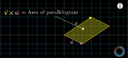
Geometric interpretation: Area of the parallelogram formed by two vectors (in two dimensional space)
几何意义(二维空间):两个向量所围成平行四边形的面积If v ⃗ \vec{v}vis on the right ofw ⃗ \vec{w}w, the product is positive; otherwise, the product is negative.
若 v ⃗ \vec{v}v 位于 w ⃗ \vec{w}w的右侧,则叉积为正;反之则为负。v ⃗ × w ⃗ = − w ⃗ × v ⃗ \vec{v} \times \vec{w} = -\vec{w} \times \vec{v}v×w=−w×v
Numeric calculation
数值计算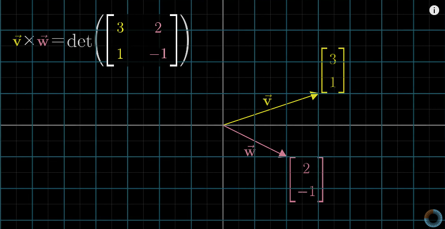
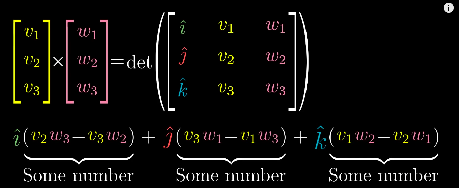
But the actual results of a cross product of two vectors is actually another vector, which is perpendicular to the parallelogram with length equals to the area of the parallelogram and direction is decided by the “right-hand rule”
但在三维空间中,两个向量叉积的结果是另一个向量:该向量与原两向量围成的平行四边形所在平面垂直,长度等于平行四边形的面积,方向由“右手定则”确定
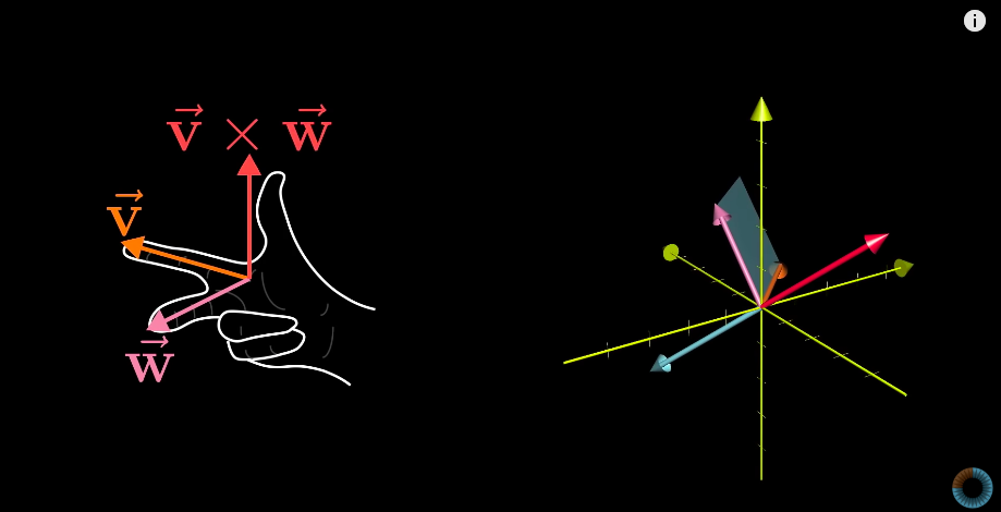
Cross products in the light of linear transformations
从线性变换视角看叉积
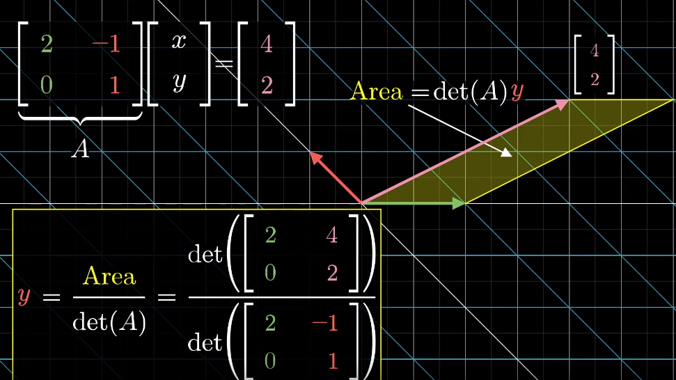
Cramer’s rule, explained geometrically
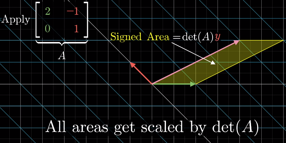
克莱姆法则的几何解释
The solution to the system of equations is given by the Cramer’s rule:
线性方程组的解可通过克莱姆法则求得,公式如下: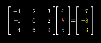
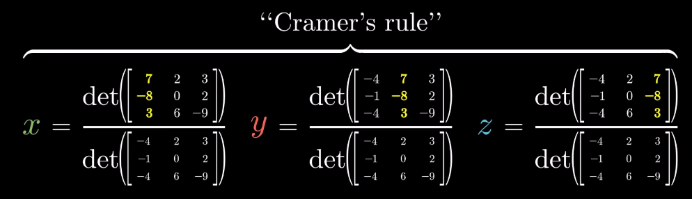
Derivation of Cramer’s rule
克莱姆法则的推导思路Any vectory → \overrightarrow{y}y (e.g. [ x y ] \begin{bmatrix}x\\y\end{bmatrix}[xy]) can define asignedarea (2D) or a “volume” (3D or above) with the basis vectors and the area/volume can be expressed by the coordinate ofx xx or y yy axis
任意向量 y → \overrightarrow{y}y(如 [ x y ] \begin{bmatrix}x\\y\end{bmatrix}[xy])可与基向量围成一个有向面积(二维)或体积(三维及以上),该面积/体积可通过向量在x xx 轴或 y yy轴上的坐标分量表示When applying a linear transformation to the vector, above area/volume is scaled by the determinant of the transformation matrix
对向量施加线性变换后,上述面积/体积会按变换矩阵的行列式值进行缩放The resulting vector also defines an area/volume, which can be calculated as the determinant of a matrix based on the transformation matrix and replacing one of its column by the resulting vector (which one to replace is dependent on which basis vector the original area is calculated from)
基于哪个基向量计算的)就是变换后的向量同样会围成一个面积/体积,该面积/体积可通过以下方式计算:以原变换矩阵为基础,将其中一列替换为变换后的向量,再计算新矩阵的行列式(替换哪一列,取决于原面积/体积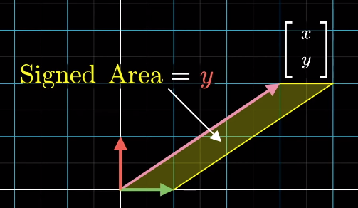
Change of basis
基变换
Eigenvectors and eigenvalues
特征向量与特征值
Many vectors get knocked out of their spans after linear transformation, but some do remain on their spans (meaning only stretch or squish effect is applied to them)
多数向量在经过线性变换后会偏离自身的张成空间,但部分向量仍会留在自身的张成空间内(即仅受到拉伸或压缩,方向不变)Those special vectors that remain on their span after linear transformation areeigenvectorsof the transformation
这些经过线性变换后仍留在自身张成空间内的特殊向量,称为该变换的特征向量Eigenvaluesare just the factors that define how much stretch/squish is applied to the eigenvectors in the linear transformation
特征值衡量线性变换对特征向量拉伸或压缩程度的系数就是则A v → = λ v → A\overrightarrow{v} = \lambda\overrightarrow{v}Av=λv
where v → \overrightarrow{v}vis the eigenvector of transformationA AA and λ \lambdaλis the eigenvalue corresponds to the eigenvector
其中,v → \overrightarrow{v}v 是变换 A AA的特征向量,λ \lambdaλ是该特征向量对应的特征值How to solve above equation?
如何求解上述方程?It can be thought as in the linear transformation, all the base vectors are multiplied by a constantλ \lambdaλ:
可将其理解为:存在一个线性变换,所有基向量都被常数λ \lambdaλ缩放,该变换的矩阵表示为:
λ I \lambda \mathbb{I}λI
(其中 I \mathbb{I}I为单位矩阵)
- Then the equation becomes
此时原方程可改写为
A v → = λ I v → ( A − λ I ) v → = 0 → \begin{aligned} A\overrightarrow{v} &= \lambda\mathbb{I}\overrightarrow{v} \\ (A - \lambda\mathbb{I}) \overrightarrow{v} &= \overrightarrow{0} \end{aligned}Av(A−λI)v=λIv=0
This leads to the fact that
要使非零向量v → \overrightarrow{v}v满足上述方程,需满足
det ( A − λ I ) = 0 \det(A - \lambda\mathbb{I}) = 0det(A−λI)=0
(即矩阵 ( A − λ I ) (A - \lambda\mathbb{I})(A−λI)的行列式为 0)
Geometric application: 3D rotation. The eigenvector is the axis of rotation
几何应用:三维旋转。此时特征向量对应旋转轴(旋转轴上的向量经旋转后方向不变,仅可能缩放)Some transformations may have more than one eigenvector/eigenvalue but some may have no eigenvector/eigenvalue, e.g. rotation in 2D space
部分线性变换可能存在多个特征向量与特征值,但也有变换不存在特征向量与特征值,例如二维空间中的旋转变换(除零向量外,所有向量旋转后都会偏离原张成空间)It’s also possible that a single eigenvalue has more than a single eigenvector, it can have a line full of eigenvectors, e.g. in Shear transformation the eigenvalue is 1 and all the vectors on the x-axis are its eigenvectors; or a transformation that scales the space by a constant, there is only one eigenvalue but infinite numbers of eigenvectors
其特征向量。就是单个特征值也可能对应多个特征向量,甚至一整条直线上的向量都是其特征向量。例如:剪切变换中,特征值 1 对应的特征向量是所有沿 x 轴的向量;再如空间整体缩放变换,仅有一个特征值,但所有非零向量都Eigenbasis: the basis vectors are also eigenvectors of the linear transformation.
特征基:指一组基向量,且这组基向量均为某个线性变换的特征向量。It comes with the transformation with diagonal matrices, where the diagonal values are the eigenvalues.
若线性变换的矩阵为对角矩阵,则该矩阵的基向量(即标准基向量)就是特征基,对角线上的元素就是对应的特征值。What if the original basis vectors are not eigenvectors? Change the coordinate system so that the eigenvectors become basis vectors.
若原基向量不是特征向量,如何处理?可依据改变坐标系,使特征向量成为新的基向量,具体步骤如下:Make those eigenvectors as columns of a matrix,known as the change of basis matrix,
将这些特征向量作为列向量构成一个矩阵,该矩阵称为基变换矩阵,记为 P PP;Sandwich the original transformation matrix with the inverse of the change of basis matrix and itself: the result will be the same transformation but using the new coordinate system and this (sandwich) matrix is guaranteed to be diagonal.
用基变换矩阵P PP 及其逆矩阵 P − 1 P^{-1}P−1对原变换矩阵A AA进行“夹逼”运算(即P − 1 A P P^{-1}APP−1AP):运算结果代表同一线性变换在新坐标系(以特征向量为基)下的矩阵,且该矩阵一定是对角矩阵;The column in the resulting diagonal matrix are the eigenbasis
上述对角矩阵的列向量即为特征基,对角线上的元素为对应的特征值。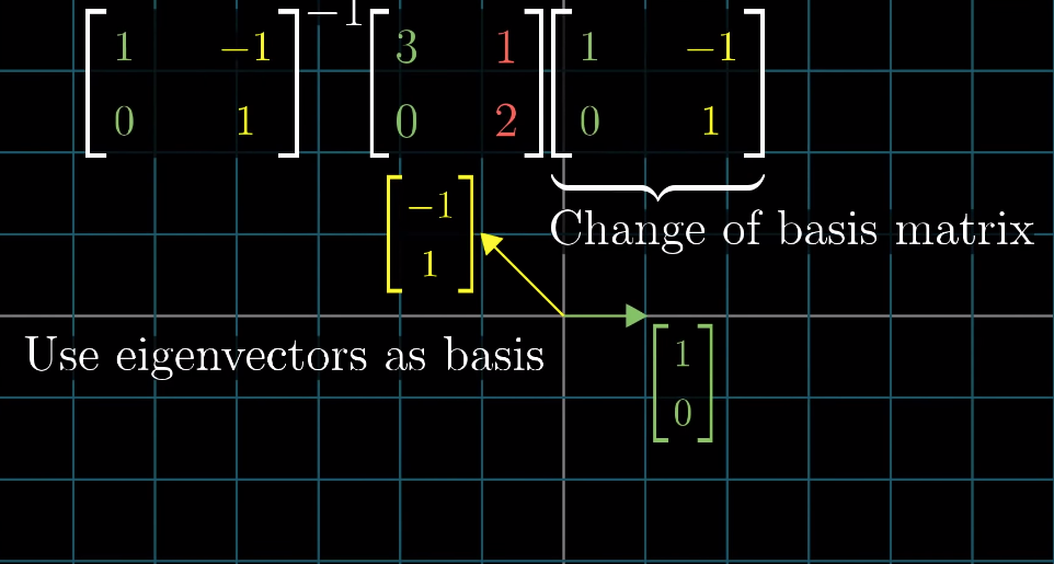
This trick can be used to calculate then nnth power of a matrix that is not diagonal
该方法可用于计算非对角矩阵的n nn 次幂:由于 ( P − 1 A P ) n = P − 1 A n P (P^{-1}AP)^n = P^{-1}A^nP(P−1AP)n=P−1AnP,因此 A n = P ( P − 1 A P ) n P − 1 A^n = P(P^{-1}AP)^nP^{-1}An=P(P−1AP)nP−1,而对角矩阵的n nn次幂可直接通过对角元素求n nn次幂得到,计算更简便。NOTE: this manipulation is not always feasible, when the existing eigenvectors are not enough to span the entire/full space then it’s not feasible.
注:该方法并非总能实现。若现有特征向量不足以张成整个空间(即矩阵不可对角化),则无法凭借这种方式将原矩阵转化为对角矩阵。
via:
线性代数的艺术.pdf
http://eagle.qlintech.cn/upload/2024/12/线性代数的艺术.pdfEssence of linear algebra — Study Notes
https://askming.github.io/study_notes/Math/Course-Essence of linear algebra.html


 浙公网安备 33010602011771号