A Gentle Introduction to Graph Neural Networks 阅读报告

一、图的基本介绍

Graphs are all around us; real world objects are often defined in terms of their connections to other things. A set of objects, and the connections between them, are naturally expressed as a graph. Researchers have developed neural networks that operate on graph data (called graph neural networks, or GNNs) for over a decade[2]. Recent developments have increased their capabilities and expressive power. We are starting to see practical applications in areas such as antibacterial discovery [3], physics simulations [4], fake news detection [5], traffic prediction [6] and recommendation systems [7].

我们身边到处都是图表;现实世界中的对象通常是根据它们与其他事物的联系来定义的。一组对象以及它们之间的联系自然地表示为图形。研究人员已经开发了操作图数据的神经网络(称为图神经网络，或GNNs)十多年了。最近的发展提高了它们的能力和表达能力。我们开始看到图神经网络在抗菌药物的发现[3]、物理模拟[4]、假新闻检测[5]、流量预测[6]和推荐系统[7]等领域的实际应用.

This article explores and explains modern graph neural networks. We divide this work into four parts. First, we look at what kind of data is most naturally phrased as a graph, and some common examples. Second, we explore what makes graphs different from other types of data, and some of the specialized choices we have to make when using graphs. Third, we build a modern GNN, walking through each of the parts of the model, starting with historic modeling innovations in the field. We move gradually from a bare-bones implementation to a state-of-the-art GNN model. Fourth and finally, we provide a GNN playground where you can play around with a real-word task and dataset to build a stronger intuition of how each component of a GNN model contributes to the predictions it makes.

该文章主要目的是探索现代图神经网络，主要包含以下四块

1. 讨论什么数据适合表示成一张图
2. 什么使得图不同于其他的数据，以及哪些情况我们必须用图神经网络
3. 构建了一个GNN，从这个模型具有历史性的创新开始，讨论这个模型的每一个模块
4. 搭建了一个平台，让人们体验GNN

To start, let’s establish what a graph is. A graph represents the relations (edges) between a collection of entities (nodes).

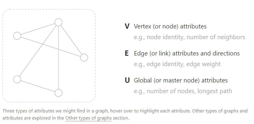
首先，我们先直观的感受一下什么是图，一张图表示的是一个实体（点）集合中的一些关系（边）。一张图包含以下的三个要素：

• 点（Vertex / node）信息，例如，点密度，邻居的数量
• 边（Edge / link）信息，例如，边密度，边权重
• 全局（Global / master node）信息，例如，点的数量，最长路径

To further describe each node, edge or the entire graph, we can store information in each of these pieces of the graph.

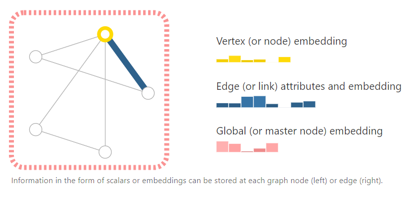
我们可以使用向量来存储图的要素信息，例如对每一个顶点，我们可以使用一个6位向量来存储，每一条边使用8位向量存储，全局信息，使用5位向量存储（文中未在此处提到每一位对应的数据是什么，但是可以假设，一个点向量可以包含点密度、邻居数量、边数量等）

We can additionally specialize graphs by associating directionality to edges (directed, undirected).

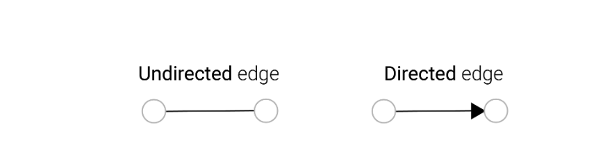
更进一步，图中的边可以分为有方向以及无方向的，一条 \(A\rightarrow B\) 有方向的边表示存在信息从A指向B,而一条 \(A-B\) 无方向的边，可以视为A到B之间存在两条有方向的边\(A\rightleftharpoons B\)。

二、数据如何表现为图

You’re probably already familiar with some types of graph data, such as social networks. However, graphs are an extremely powerful and general representation of data, we will show two types of data that you might not think could be modeled as graphs: images and text. Although counterintuitive, one can learn more about the symmetries and structure of images and text by viewing them as graphs,, and build an intuition that will help understand other less grid-like graph data, which we will discuss later.

您可能已经熟悉了某些类型的图数据，例如社交网络。然而，图是一种非常强大和通用的数据表示，我们将展示两种您可能认为不能建模为图的数据:图像和文本。尽管违反直觉，但人们可以通过将图像和文本视为图表来了解更多关于它们的对称性和结构，并建立一种直觉，这将有助于理解其他不太像网格的图表数据，我们将在后面讨论。

2.1 如果将图片表示为图

We typically think of images as rectangular grids with image channels, representing them as arrays (e.g., 244x244x3 floats). Another way to think of images is as graphs with regular structure, where each pixel represents a node and is connected via an edge to adjacent pixels. Each non-border pixel has exactly 8 neighbors, and the information stored at each node is a 3-dimensional vector representing the RGB value of the pixel.
 
A way of visualizing the connectivity of a graph is through its adjacency matrix. We order the nodes, in this case each of 25 pixels in a simple 5x5 image of a smiley face, and fill a matrix of \(n_{nodes} \times n_{nodes}\) with an entry if two nodes share an edge. Note that each of these three representations below are different views of the same piece of data.

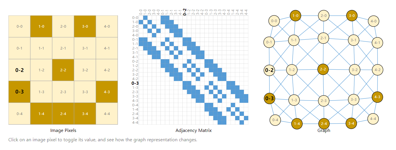
以上图为例，左侧图a是最常见的将一张图表示为一个矩阵；中间图b则将图表示邻接矩阵（邻接矩阵的坐标轴分别表示图a中的每一个像素，而矩阵中每一个蓝色的点则表示对应的两个像素相邻，例如 0-0 与 1-1 对角相邻）；右侧的图c则是图片的图表示，其中每一个点表示一个像素，每一条边表示它的两个像素是否相邻。

2.2 将文本表现为图

We can digitize text by associating indices to each character, word, or token, and representing text as a sequence of these indices. This creates a simple directed graph, where each character or index is a node and is connected via an edge to the node that follows it.

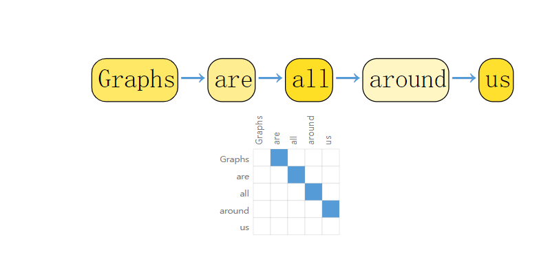
将文本表达为图最直接的方式就是将每个单词组成结点，然后使用有向边将前一个单词连向后一个单词。

Of course, in practice, this is not usually how text and images are encoded: these graph representations are redundant since all images and all text will have very regular structures. For instance, images have a banded structure in their adjacency matrix because all nodes (pixels) are connected in a grid. The adjacency matrix for text is just a diagonal line, because each word only connects to the prior word, and to the next one.

上述两个例子都非常直观，但是事实上当真实应用时图很有可能并不是这样构建的，因为上述两种方式构成的图都具有相同的结构

2.3 更真实的图表示方法

Graphs are a useful tool to describe data you might already be familiar with. Let’s move on to data which is more heterogeneously structured. In these examples, the number of neighbors to each node is variable (as opposed to the fixed neighborhood size of images and text). This data is hard to phrase in any other way besides a graph.

下面我们将给出一些例子，给出更加真实的图的表示，对于某些数据，你很难使用除图以外的数据结构来表示实体与实体之间的关系

Molecules as graphs. Molecules are the building blocks of matter, and are built of atoms and electrons in 3D space. All particles are interacting, but when a pair of atoms are stuck in a stable distance from each other, we say they share a covalent bond. Different pairs of atoms and bonds have different distances (e.g. single-bonds, double-bonds). It’s a very convenient and common abstraction to describe this 3D object as a graph, where nodes are atoms and edges are covalent bonds. Here are two common molecules, and their associated graphs.[8]

将分子表示为图，将没一个原子视为点，同时将原子之间的键视为边

Social networks as graphs. Social networks are tools to study patterns in collective behaviour of people, institutions and organizations. We can build a graph representing groups of people by modelling individuals as nodes, and their relationships as edges.

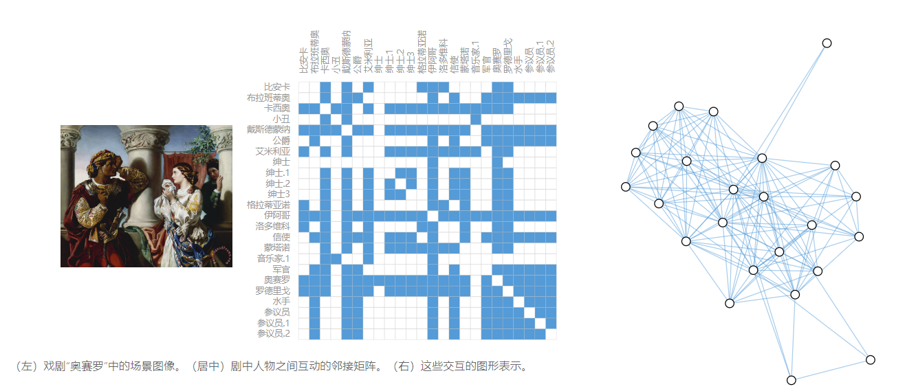
将社交网络表示为图，上图是戏剧奥赛罗中的人物关系表，其中每一个人表示为一个节点，而人之间的关系表现为一条边。

Citation networks as graphs. Scientists routinely cite other scientists’ work when publishing papers. We can visualize these networks of citations as a graph, where each paper is a node, and each directed edge is a citation between one paper and another. Additionally, we can add information about each paper into each node, such as a word embedding of the abstract. (see , , ). [9] [10] [11]

论文引文网络，将每一篇文献视为结点，将引用视为一条有向边

2.4 现实最中的一些图

Other examples. In computer vision, we sometimes want to tag objects in visual scenes. We can then build graphs by treating these objects as nodes, and their relationships as edges. Machine learning models, programming code and math equations can also be phrased as graphs, where the variables are nodes, and edges are operations that have these variables as input and output. You might see the term “dataflow graph” used in some of these contexts.[12][13]
 
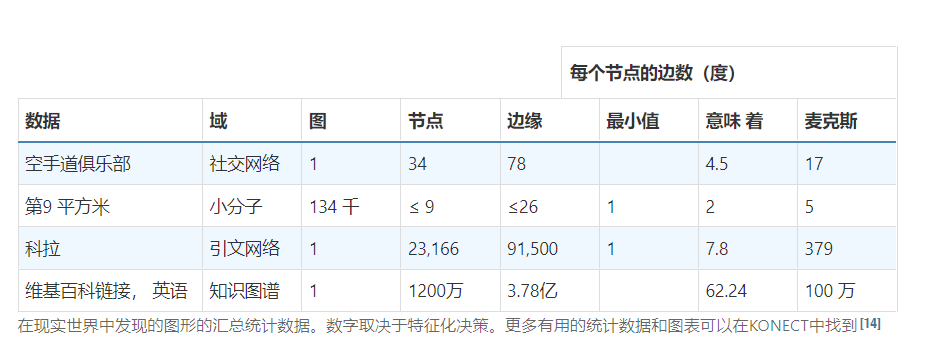
The structure of real-world graphs can vary greatly between different types of data — some graphs have many nodes with few connections between them, or vice versa. Graph datasets can vary widely (both within a given dataset, and between datasets) in terms of the number of nodes, edges, and the connectivity of nodes.

3. 图上定义的任务

We have described some examples of graphs in the wild, but what tasks do we want to perform on this data? There are three general types of prediction tasks on graphs: graph-level, node-level, and edge-level.
 
In a graph-level task, we predict a single property for a whole graph. For a node-level task, we predict some property for each node in a graph. For an edge-level task, we want to predict the property or presence of edges in a graph.
 
For the three levels of prediction problems described above (graph-level, node-level, and edge-level), we will show that all of the following problems can be solved with a single model class, the GNN. But first, let’s take a tour through the three classes of graph prediction problems in more detail, and provide concrete examples of each.

在定义了图后，我们可以定义在图上三种类型的任务：图级任务，节点级任务，边级任务。

3.1 图级任务

In a graph-level task, our goal is to predict the property of an entire graph. For example, for a molecule represented as a graph, we might want to predict what the molecule smells like, or whether it will bind to a receptor implicated in a disease.

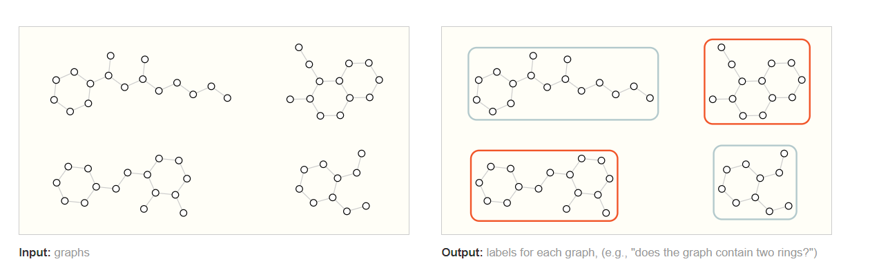
This is analogous to image classification problems with MNIST and CIFAR, where we want to associate a label to an entire image. With text, a similar problem is sentiment analysis where we want to identify the mood or emotion of an entire sentence at once.

图级任务负责预测整个图的全局属性，例如，对于表示为图的分子
我们可以预测该分子是否存在刺激性气味。对于表示为图的图像我们可以预测整张图像的上标签或物体。对于表示为图的文本，我们希望可以识别整个句子的情绪或情感。

3.2 节点级任务

Node-level tasks are concerned with predicting the identity or role of each node within a graph.
 
A classic example of a node-level prediction problem is Zach’s karate club. The dataset is a single social network graph made up of individuals that have sworn allegiance to one of two karate clubs after a political rift. As the story goes, a feud between Mr. Hi (Instructor) and John H (Administrator) creates a schism in the karate club. The nodes represent individual karate practitioners, and the edges represent interactions between these members outside of karate. The prediction problem is to classify whether a given member becomes loyal to either Mr. Hi or John H, after the feud. In this case, distance between a node to either the Instructor or Administrator is highly correlated to this label.[15]

Following the image analogy, node-level prediction problems are analogous to image segmentation, where we are trying to label the role of each pixel in an image. With text, a similar task would be predicting the parts-of-speech of each word in a sentence (e.g. noun, verb, adverb, etc).

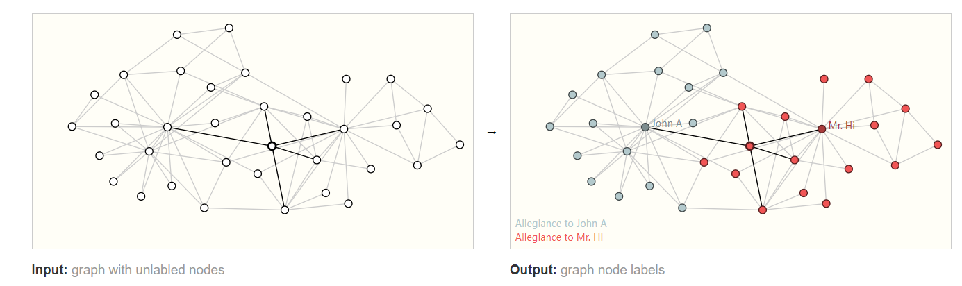
节点级任务扶着预测图形中每个节点的标识或类别。一个经典的例子是存在一个社交网络图，在选举时我们预测该社交网络中每一个人(节点)的政治倾向。对于表示为图的图像，图可以预测图像中的每个像素的类别用于语义分割或实例分割。对于表示为图的文本则可以预测文本中每一个词的词性(名词、动词或副词)。

3.3 边级任务

The remaining prediction problem in graphs is edge prediction.
 
One example of edge-level inference is in image scene understanding. Beyond identifying objects in an image, deep learning models can be used to predict the relationship between them. We can phrase this as an edge-level classification: given nodes that represent the objects in the image, we wish to predict which of these nodes share an edge or what the value of that edge is. If we wish to discover connections between entities, we could consider the graph fully connected and based on their predicted value prune edges to arrive at a sparse graph.

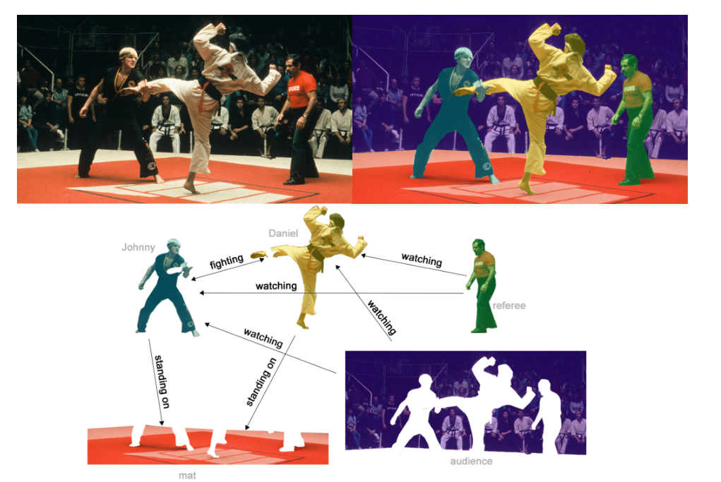
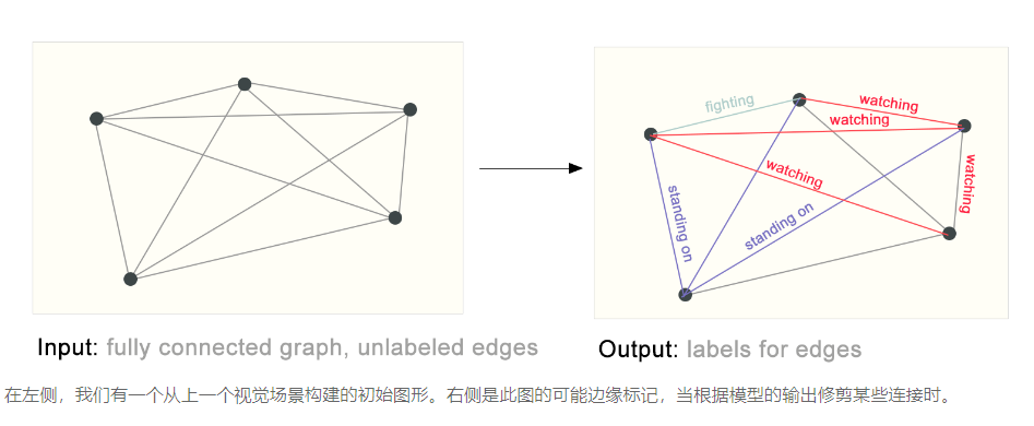
边级任务的一个例子是图像的场景理解，除了识别图像中的对象外，边级任务还可以预测图中各个对象的关系。例如图片中的场景预测任务，通过节点级任务，我们首先可以对图片中的每一个像素的类别，分类出图像中每一个实体，然后通过边级预测任务识别出每一个节点之间的关系（首先图像中的每一个像素与其相邻的像素之间存在边，经过预测后所有像素的边不变，但是为每一条边都存在了置信度的预测值，经过剪裁后得到各个实体的关系。）

3.4 在机器学习中使用图的挑战

So, how do we go about solving these different graph tasks with neural networks? The first step is to think about how we will represent graphs to be compatible with neural networks.
 
Machine learning models typically take rectangular or grid-like arrays as input. So, it’s not immediately intuitive how to represent them in a format that is compatible with deep learning. Graphs have up to four types of information that we will potentially want to use to make predictions: nodes, edges, global-context and connectivity. The first three are relatively straightforward: for example, with nodes we can form a node feature matrix N by assigning each node an index i and storing the feature for nodei in N. While these matrices have a variable number of examples, they can be processed without any special techniques.
 
However, representing a graph’s connectivity is more complicated. Perhaps the most obvious choice would be to use an adjacency matrix, since this is easily tensorisable. However, this representation has a few drawbacks. From the example dataset table, we see the number of nodes in a graph can be on the order of millions, and the number of edges per node can be highly variable. Often, this leads to very sparse adjacency matrices, which are space-inefficient.
 
Another problem is that there are many adjacency matrices that can encode the same connectivity, and there is no guarantee that these different matrices would produce the same result in a deep neural network (that is to say, they are not permutation invariant).
 
For example, the Othello graph from before can be described equivalently with these two adjacency matrices. It can also be described with every other possible permutation of the nodes.

机器学习模型通常采用张量或向量数据作为输入。因此，如何将图表示为机器学习兼容的数据是一个不小的挑战。图形中包含四种类型我们希望进行预测的信息：节点信息、边信息、全局信息和图的连通性（哪些节点是相连的），前三种都可以像上文描述的使用向量进行表示（以节点为例，我们可以用一个向量表示一个节点，然后这些节点向量组成一个特征矩阵\(N\)），但是对于图的连通性则是一个麻烦的问题。

如果我们使用图的邻接矩阵，它的确能够清晰的表示点与点之间的连接性，但是这个矩阵高度依赖于节点的顺序，对于同一个图，节点的顺序不一致我们就会获得完全不同的邻接矩阵（如上图），但是使用机器学习对于图的处理时我们希望对于同一个图都能获得一致的处理结果，而无关节点的排列顺序。另外邻接矩阵往往是一个相当稀疏的矩阵，对于节点较多的图而言，这个矩阵会非常巨大，因此也会对计算内存产生不小的负担。

p.s. 这里提到的“节点的顺序”并不是指对于同一个节点我们可以将其命名为‘A’ 也可以将其名为‘B’ 然后我们 'A-B-C-D' 顺序摆放邻接矩阵的时候会产生不同的邻接矩阵。而是我们固定将某个节点命名为‘A’，然后我们按照不同顺序摆放邻接矩阵时产生了不一样的邻接矩阵。例如，在节点名称固定后按照'A-B-C-D' 和按照 'B-A-D-C' 摆放的邻接矩阵时不一致的

For example, the Othello graph from before can be described equivalently with these two adjacency matrices. It can also be described with every other possible permutation of the nodes.

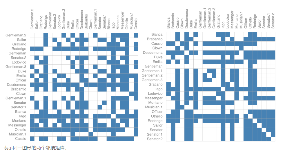
例如上图描述的是戏剧奥赛罗的人物关系图，对于同一张图，不同的人物顺序产生了完全不同的邻接矩阵。

The example below shows every adjacency matrix that can describe this small graph of 4 nodes. This is already a significant number of adjacency matrices–for larger examples like Othello, the number is untenable.

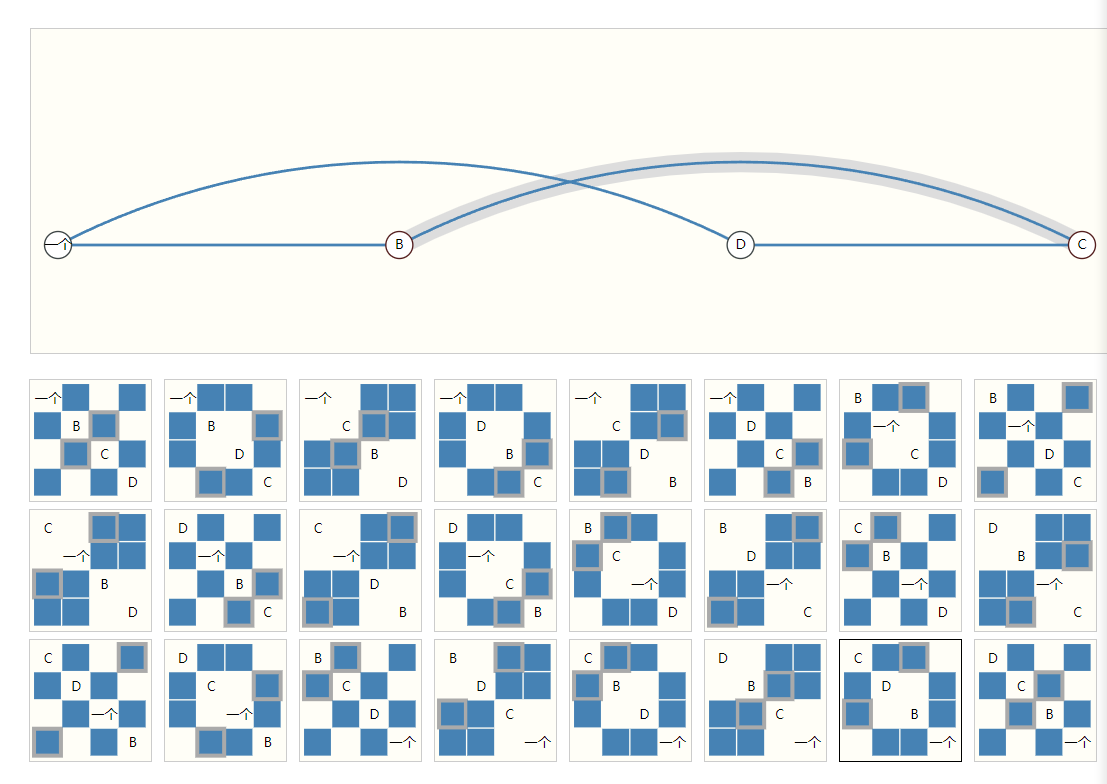
上面这个例子显示了一张四节点的图，在不同节点排序的情况下能产生24个表示同样意义的邻接矩阵。

One elegant and memory-efficient way of representing sparse matrices is as adjacency lists. These describe the connectivity of edge \(e^k\) between nodes \(n_i\) and \(n_j\) as a tuple (i,j) in the k-th entry of an adjacency list. Since we expect the number of edges to be much lower than the number of entries for an adjacency matrix (\(n^2_{nodes}\)), we avoid computation and storage on the disconnected parts of the graph.
 
To make this notion concrete, we can see how information in different graphs might be represented under this specification:

 
It should be noted that the figure uses scalar values per node/edge/global, but most practical tensor representations have vectors per graph attribute. Instead of a node tensor of size \([n_{nodes}]\) we will be dealing with node tensors of size \([n_{nodes},node_{dim}]\). Same for the other graph attributes.

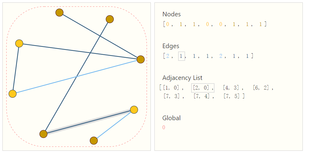
为了解决上述问题，使用邻接列表是个合适的方案，首先，在描述连连性时，相同的图产生的邻接列表是一致的，不会产生同一个图有多个连通性描述特征的问题。其次，图的连接往往是稀疏的，使用图的邻接列表可以降低存储的需求，同时也可以避免大量非连接的数据加入到计算中。上图，给出了一个邻接列表的例子，使用一个二元组来表示节点之间的连接性。为了简便图中使用了标量来表示节点、边、全局特征，实际时需要将这些标量替换为特征向量。

4. 图神经网络

Now that the graph’s description is in a matrix format that is permutation invariant, we will describe using graph neural networks (GNNs) to solve graph prediction tasks. A GNN is an optimizable transformation on all attributes of the graph (nodes, edges, global-context) that preserves graph symmetries (permutation invariances). We’re going to build GNNs using the “message passing neural network” framework proposed by Gilmer et al. using the Graph Nets architecture schematics introduced by Battaglia et al. GNNs adopt a “graph-in, graph-out” architecture meaning that these model types accept a graph as input, with information loaded into its nodes, edges and global-context, and progressively transform these embeddings, without changing the connectivity of the input graph.[18][19]

GNN是对图形的所有特征（节点、边、全局信息）进行的可优化变换，经过变换后仍然能够保留图的对称性(即改变节点的顺序不会导致结果的改变/排列不变性)。本文使用Gilmer等人提出的消息传递神经网络框架构建GNN，这个框架表意味着GNN接受一个图并且输出也是一个图。在训练的过程中节点、边、全局信息特征逐步被优化，但是图的连接性是不变的。

4.1 最简单的GNN

With the numerical representation of graphs that we’ve constructed above (with vectors instead of scalars), we are now ready to build a GNN. We will start with the simplest GNN architecture, one where we learn new embeddings for all graph attributes (nodes, edges, global), but where we do not yet use the connectivity of the graph.
 
For simplicity, the previous diagrams used scalars to represent graph attributes; in practice feature vectors, or embeddings, are much more useful.
This GNN uses a separate multilayer perceptron (MLP) (or your favorite differentiable model) on each component of a graph; we call this a GNN layer. For each node vector, we apply the MLP and get back a learned node-vector. We do the same for each edge, learning a per-edge embedding, and also for the global-context vector, learning a single embedding for the entire graph.

我们利用上面定义的数据格式来构造如上图所示的最简单的图神经网络，我们拥有若5个节点的特征向量，不妨假设每个结点的向量长度为11，有6条边对应6个边特征向量，假设长度为7，假设全局特征向量有3个，每个长度长为5。考虑最简单的情况，我们可以构造三个多层感知机输入分别为11,7,5个结点，用于做点、边、全局特征的变换，命名为\(MLP_{node},MLP_{edge},MLP_{global}\)。图神经网络对点、边、全局分别做训练，变换或预测。经过处理后可以点、边、全局特征都可以获得一个新的数值。对于某些应用，这些特征可能就是想要的特征，例如社交网络图中我们可以通过某条边的置信度来预测两个人是否认识；对于另外一些应用，图中的特征可能还需要外接一个全连接层进行分类，例如对在一次选举中，对某人的选择进行预测就可能需要将每个人的特征放入一个全连接层获得具体的分类(对于是否需要全连接层的加入，个人目前认为主要和需要预测的特征有关，如果需要预测的特征属于对象的属性，例如人的年龄等，那么对节点的属性进行预测即可不需要加入全连接层。如果需要预测的特征不是对象本身的属性，例如选举倾向，那么应该加入全连接层)。

P.S.对于一个图神经网络可以做训练样本有可能为一个完整的图（分子图）也有可能为一个点和边的样本(社交网络图),以前者为例，训练时将图中的节点逐个拿出放进\(MLP_{node}\)对其进行训练，然后在取出逐条边放进MLP_{edge}，对其进行训练……

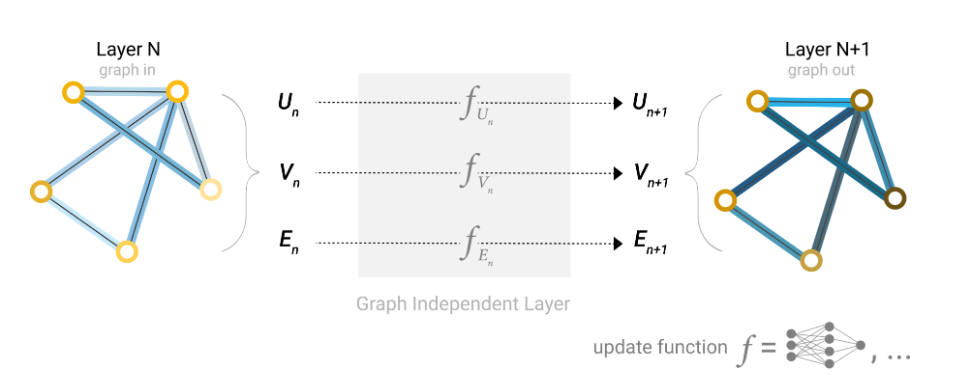
As is common with neural networks modules or layers, we can stack these GNN layers together.
 
Because a GNN does not update the connectivity of the input graph, we can describe the output graph of a GNN with the same adjacency list and the same number of feature vectors as the input graph. But, the output graph has updated embeddings, since the GNN has updated each of the node, edge and global-context representations.

像上面的三个多层感知机(MLP),我们可以当成普通图神经网络中的一层，类似于其他的神经网络，将多层堆叠在一起，就构成了图神经网络。值的注意的是，图神经网络不会更新输入图的连通性，因此输出图的连通性与输入是一致的，但是图中的特征已经被更新了。对于一些需要预测节点是否连通的应用，我们可以通过给边特征设置置信度来实现，经过预测后，对边置信度较低的边进行裁剪，就可以判断节点是否相连。

4.2 汇集(池化)信息的GNN

We have built a simple GNN, but how do we make predictions in any of the tasks we described above?
 
We will consider the case of binary classification, but this framework can easily be extended to the multi-class or regression case. If the task is to make binary predictions on nodes, and the graph already contains node information, the approach is straightforward — for each node embedding, apply a linear classifier.

上面我们已经构造了一个最简单的GNN了，但是我们如何在上述GNN中进行预测呢，我们以二元分类为例，如果某个任务需要对节点进行二分类，并且节点中已经包含了全部的所需的信息，那么我们将经过图神经网络处理后的点特征传入到全连接层或线性分类器中，对该节点进行分类。

However, it is not always so simple. For instance, you might have information in the graph stored in edges, but no information in nodes, but still need to make predictions on nodes. We need a way to collect information from edges and give them to nodes for prediction. We can do this by pooling. Pooling proceeds in two steps:
 
1.For each item to be pooled, gather each of their embeddings and concatenate them into a matrix.
 
2.The gathered embeddings are then aggregated, usually via a sum operation.
 
For a more in-depth discussion on aggregation operations go to the Comparing aggregation operations section.
We represent the pooling operation by the letter ρ, and denote that we are gathering information from edges to nodes as \(PE_n \rightarrow V_n\)

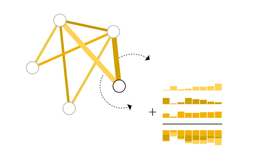
但是对于某种图，节点可能会不存储信息而将信息存储到边上，当节点上没有信息，但又要对节点进行预测，那么此时就需要通过一种方式从边缘中汇集信息，构成节点的特征，具体的汇集工作分为两步

1. 将与节点相连的边特征以及全局特征组成一个矩阵
2. 将这个矩阵进行聚合，一般是通过求和实现的

一个值得注意的问题是，汇集信息时要求点、边、全局变量维度一致，否则无法相加。例如上图右下角节点特征为空，但又需要对该节点进行预测时，就将全局变量和两个与该节点相连的边特征相加，得到汇集的结点特征。

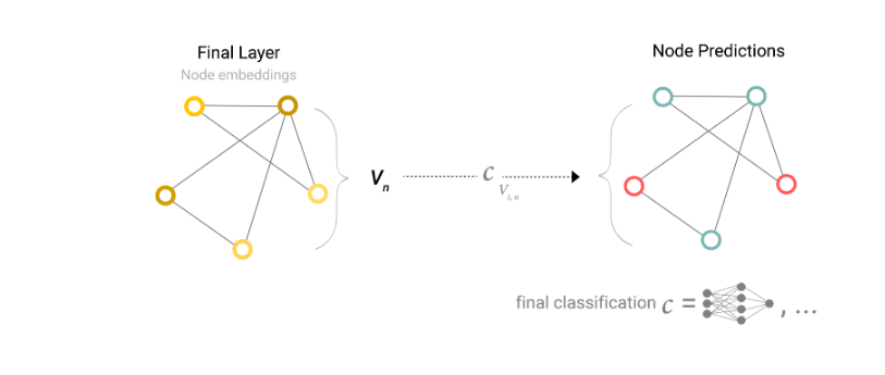
So If we only have edge-level features, and are trying to predict binary node information, we can use pooling to route (or pass) information to where it needs to go. The model looks like this.

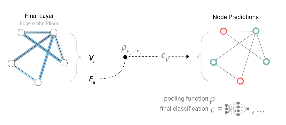
当一个图只有边特征，且又需要对节点进行预测时，整体的模型就如上图所示，首先某个节点\(V_n\)从相连的边上汇集信息\(P_{E_n\rightarrow V_n}\),然后经过一个线性分类器\(C_{V_n}\)对节点进行预测。

If we only have node-level features, and are trying to predict binary edge-level information, the model looks like this.

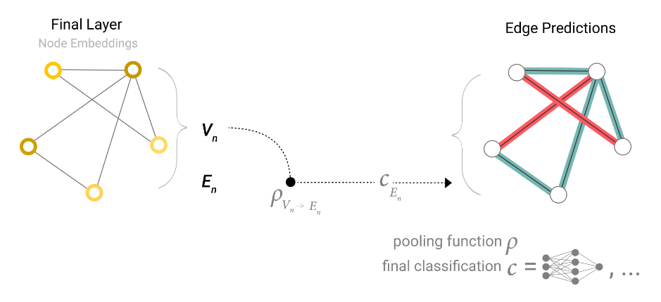
同样的，如果一个图只有节点信息，而任务需要对边进行预测时，边就可以从相连的节点中汇聚信息，整体的模型结构如上图所示

If we only have node-level features, and need to predict a binary global property, we need to gather all available node information together and aggregate them. This is similar to Global Average Pooling layers in CNNs. The same can be done for edges.

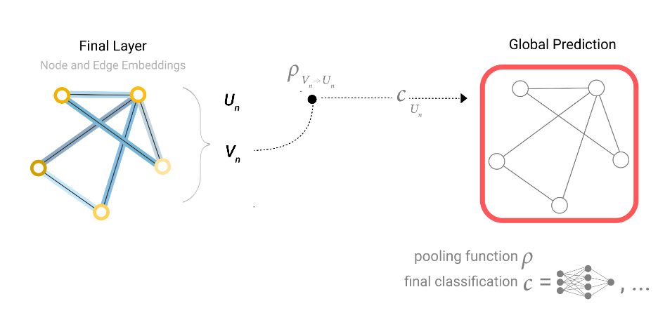
当仅有节点或边特征，而需要预测全局特征时，同样可以使用汇集信息的方法。当节点和边特征都存在时，同样可以将边和节点都汇聚在一起对全局特征进行预测。

在使用了汇聚信息方法时，只要存在一种特征就可以对其余两种特征进行预测，扩宽了GNN的适用范围

In our examples, the classification model c can easily be replaced with any differentiable model, or adapted to multi-class classification using a generalized linear model.

Now we’ve demonstrated that we can build a simple GNN model, and make binary predictions by routing information between different parts of the graph. This pooling technique will serve as a building block for constructing more sophisticated GNN models. If we have new graph attributes, we just have to define how to pass information from one attribute to another.
 
Note that in this simplest GNN formulation, we’re not using the connectivity of the graph at all inside the GNN layer. Each node is processed independently, as is each edge, as well as the global context. We only use connectivity when pooling information for prediction.

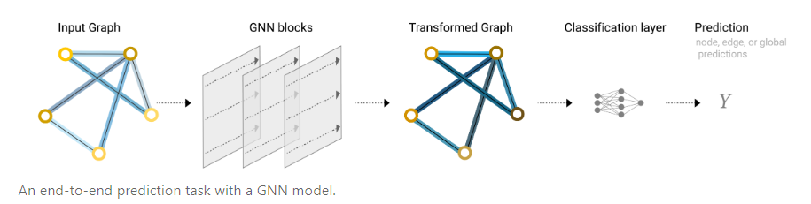
经过上述的讨论，我们可以得到一个更贴近实际的端到端图神经网络结构，首先有一个输入的图，经过若干个GNN层，其中每个层中包含三个多层感知机，获得一个输出图，这个输出图保持了输入图的连接性不变，但是内部的点、边、全局特征均产生了变化。最后根据任务需求对特征做预测时，就可以在最后加入全连接层对特征进行预测。如果缺少需要预测的特征信息就可以通过汇聚信息的方法去构造合适的特征。

上面这个图神经网络已经能够正常使用了，但是此时的图神经网络仍然具有很大的局限性。主要问题在于GNN层中没有利用到图的结构信息(连通性)，点、边、全局特征只会进入各自的MLP，导致各种信息是孤立的，与单独训练3个更深的MLP没有太大区别（除了缺失信息时）一下我们将会讨论更复杂的GNN，使得图的连接性信息得到充分利用。

4.5 信息传递的GNN

We could make more sophisticated predictions by using pooling within the GNN layer, in order to make our learned embeddings aware of graph connectivity. We can do this using message passing, where neighboring nodes or edges exchange information and influence each other’s updated embeddings.[18]
 
Message passing works in three steps:
 
1.For each node in the graph, gather all the neighboring node embeddings (or messages), which is the g function described above.
 
2.Aggregate all messages via an aggregate function (like sum).
 
3.All pooled messages are passed through an update function, usually a learned neural network.
 
Just as pooling can be applied to either nodes or edges, message passing can occur between either nodes or edges.
 
These steps are key for leveraging the connectivity of graphs. We will build more elaborate variants of message passing in GNN layers that yield GNN models of increasing expressiveness and power.

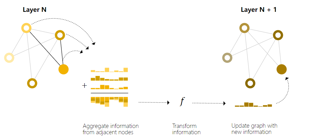
上面我们提到，在最简单的GNN时，每个节点是独立进入到MLP中的，也就是说没有利用图的连接信息。所以为了充分利用连接信息提出了传递信息的GNN，如上图所示，在每一层GNN层中，我们首先将某个节点的相邻节点的特征汇聚到该节点（求和），然后再将汇聚后的节点信息传入MLP。如图所示，需要对右下角节点进行处理时，将与其相连的两个节点加到该节点上，然后再进入到该层节点的MLP \(f\) 进行处理。

This sequence of operations, when applied once, is the simplest type of message-passing GNN layer.
 
This is reminiscent of standard convolution: in essence, message passing and convolution are operations to aggregate and process the information of an element’s neighbors in order to update the element’s value. In graphs, the element is a node, and in images, the element is a pixel. However, the number of neighboring nodes in a graph can be variable, unlike in an image where each pixel has a set number of neighboring elements.
 
By stacking message passing GNN layers together, a node can eventually incorporate information from across the entire graph: after three layers, a node has information about the nodes three steps away from it.
 
We can update our architecture diagram to include this new source of information for nodes:

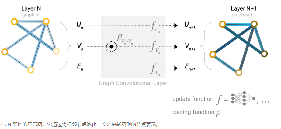
假设没一层都汇集距离为1的邻居节点的信息，那么经过三层GNN层后节点就可以获得与其距离为3的节点的信息。这就与CNN中逐步扩大感受野的原理类似了。但是有一个区别是，CNN的卷积核是对相邻像素的加权求和，但是图里的汇集信息或信息传递则只进行了求和，而没有了加权的步骤。在增加了节点的信息传递后，一个GNN层结构如上图所示，对于某个节点\(V_n\) 首先经过信息传递\(P_{V_n\rightarrow V_n}\) 后再进入MLP \(f_{V_n}\)对特征进行变换

4.6 全局特征

There is one flaw with the networks we have described so far: nodes that are far away from each other in the graph may never be able to efficiently transfer information to one another, even if we apply message passing several times. For one node, If we have k-layers, information will propagate at most k-steps away. This can be a problem for situations where the prediction task depends on nodes, or groups of nodes, that are far apart. One solution would be to have all nodes be able to pass information to each other. Unfortunately for large graphs, this quickly becomes computationally expensive (although this approach, called ‘virtual edges’, has been used for small graphs such as molecules).[18]
 
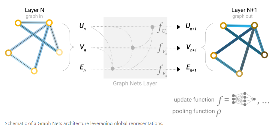
One solution to this problem is by using the global representation of a graph (U) which is sometimes called a master node or context vector. This global context vector is connected to all other nodes and edges in the network, and can act as a bridge between them to pass information, building up a representation for the graph as a whole. This creates a richer and more complex representation of the graph than could have otherwise been learned. [19][18]

到目前为止，我们获得了一个可以传递信息的GNN，但是还有一个缺陷在于当图比较大时需要非常多的GNN层才能使得两个较远节点的信息互相传递，并且GNN的计算量要比普通的CNN要高，所以这就会导致非常高的计算资源需求。因此我们考虑设置一个(虚拟的)全局节点，该全局节点与图中所有点和边相连，所有的点和边都可以利用全局节点来进行信息传递。通过这项设置，我们可以快速的实现全局的信息传递。在加上全局节点后，单个GNN层结构如上图所示。

In this view all graph attributes have learned representations, so we can leverage them during pooling by conditioning the information of our attribute of interest with respect to the rest. For example, for one node we can consider information from neighboring nodes, connected edges and the global information. To condition the new node embedding on all these possible sources of information, we can simply concatenate them. Additionally we may also map them to the same space via a linear map and add them or apply a feature-wise modulation layer, which can be considered a type of featurize-wise attention mechanism.[22]

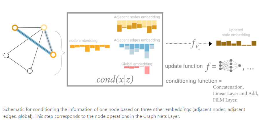
在最终的模型中，一个节点或边的特征可以在信息传递阶段，汇聚相邻节点的特征，相邻边的特征以及全局特征后在进入到MLP中进行变换，汇聚的操作可以用求和、Concat等各种方法。我们可以认为汇聚信息的操作类似于注意力机制。

5. 总结

上文简单的介绍了GNN，从图的基本对象点、边、全局特征说起，再介绍在图上定义的问题，对不同的基本对象进行预测。继而讨论在图在机器学习中存在的问题。最后引出了图神经网络GNN，呈现出一个带有信息传递的图神经网络。