

参考:https://www.kaggle.com/lavanyashukla01/how-i-made-top-0-3-on-a-kaggle-competition
导入相关的python包


import numpy as np
import pandas as pd
import datetime
import random
#plot
import seaborn as sns
import matplotlib.pyplot as plt

#model
from sklearn.ensemble import RandomForestRegressor,GradientBoostingRegressor,AdaBoostRegressor,BaggingRegressor
from sklearn.kernel_ridge import KernelRidge
from sklearn.linear_model import Ridge,RidgeCV,ElasticNet,ElasticNetCV
from sklearn.svm import SVR
from mlxtend.regressor import StackingCVRegressor
import lightgbm as lgb
from lightgbm import LGBMRegressor
from xgboost import XGBRegressor

#统计相关
from scipy.stats import skew,norm,boxcox_normmax
from scipy.special import boxcox1p

#特征预处理
from sklearn.model_selection import GridSearchCV,KFold,cross_val_score
from sklearn.metrics import mean_squared_error
from sklearn.preprocessing import OneHotEncoder,LabelEncoder,scale,StandardScaler,RobustScaler
from sklearn.decomposition import PCA
from sklearn.pipeline import make_pipeline

pd.set_option('display.max_columns',None)
import warnings
warnings.filterwarnings("ignore")
1.读取数据
train=pd.read_csv('./data/train.csv')
test=pd.read_csv('./data/test.csv')
train.shape,test.shape
((1460, 81), (1459, 80))
2.EDA
2.1 目标标签可视化
sns.set_style('darkgrid')
plt.rcParams['font.sans-serif'] = ['SimHei']
plt.rcParams['axes.unicode_minus'] = False

sns.distplot(train['SalePrice'],color='b')
plt.ylabel("frequency")
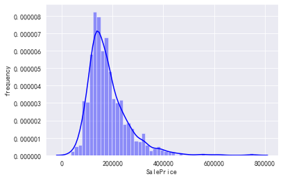
train['SalePrice'].skew(),train['SalePrice'].kurt()
(1.8828757597682129, 6.536281860064529)
- kurt:峰度系数是用来反映频数分布曲线顶端尖峭或扁平程度的指标
- skew:偏度系数是描述分布偏离对称性程度的一个特征数。当分布左右对称时,偏度系数为0。当偏度系数大于0时,即重尾在右侧时,该分布为右偏。当偏度系数小于0时,即重尾在左侧时,该分布左偏
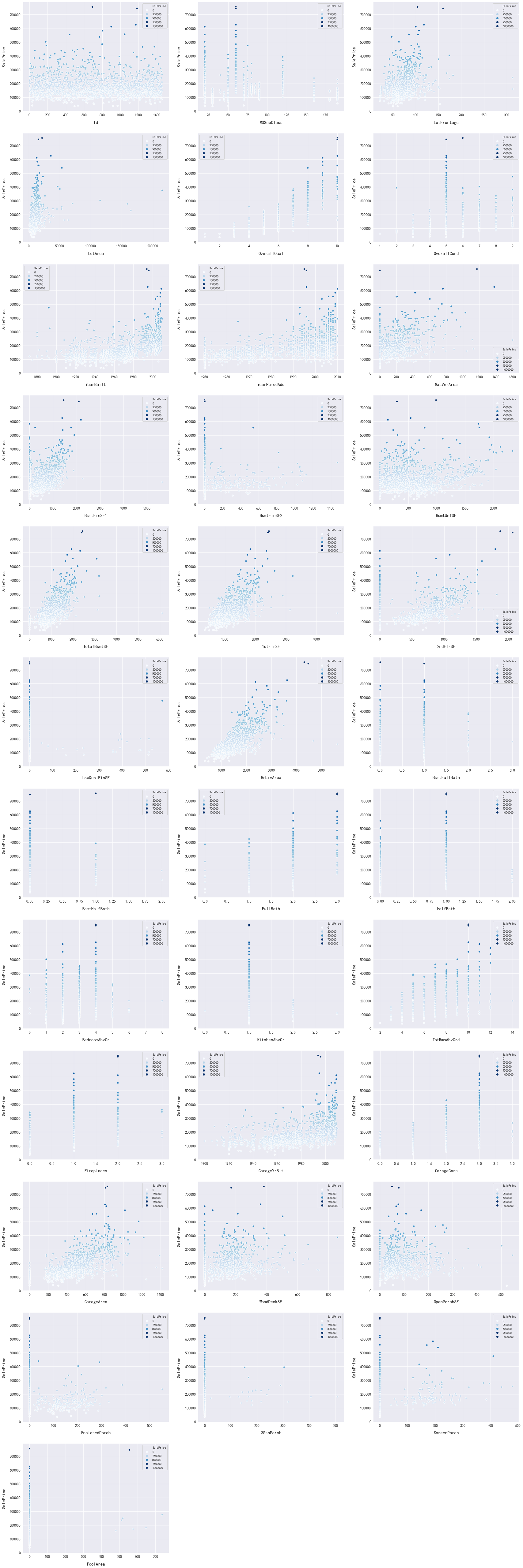
2.2 特征可视化
#画出所有数值型特征
num_dtypes=['int16','int32','int64','float16','float32','float64']
not_plot=['TotalSF','Total_Bathroom','Total_porch_sf','haspool','hasgarage','hasbsmt','hasfireplace']
num=[]
for i in train.columns:
    if train[i].dtypes in num_dtypes:
        if i in not_plot: pass
        else:num.append(i)


fig,axs=plt.subplots(ncols=2,nrows=0,figsize=(12,120))
plt.subplots_adjust(right=2)
plt.subplots_adjust(top=2)
sns.color_palette("husl",8)
for i,feature in  enumerate(list(train[num]),1):
    if(feature=='MiscVal'):
        break
    plt.subplot(len(list(num)),3,i)
    sns.scatterplot(x=feature,y='SalePrice',hue='SalePrice',palette='Blues',data=train)

    plt.xlabel('{c}'.format(c=feature),size=15,labelpad=12.5)
    plt.ylabel("SalePrice",size=15,labelpad=12.5)

    for j in range(2):
        plt.tick_params(axis='x',labelsize=12)
        plt.tick_params(axis='y',labelsize=12)
    plt.legend(loc='best',prop={'size':10})
plt.show()
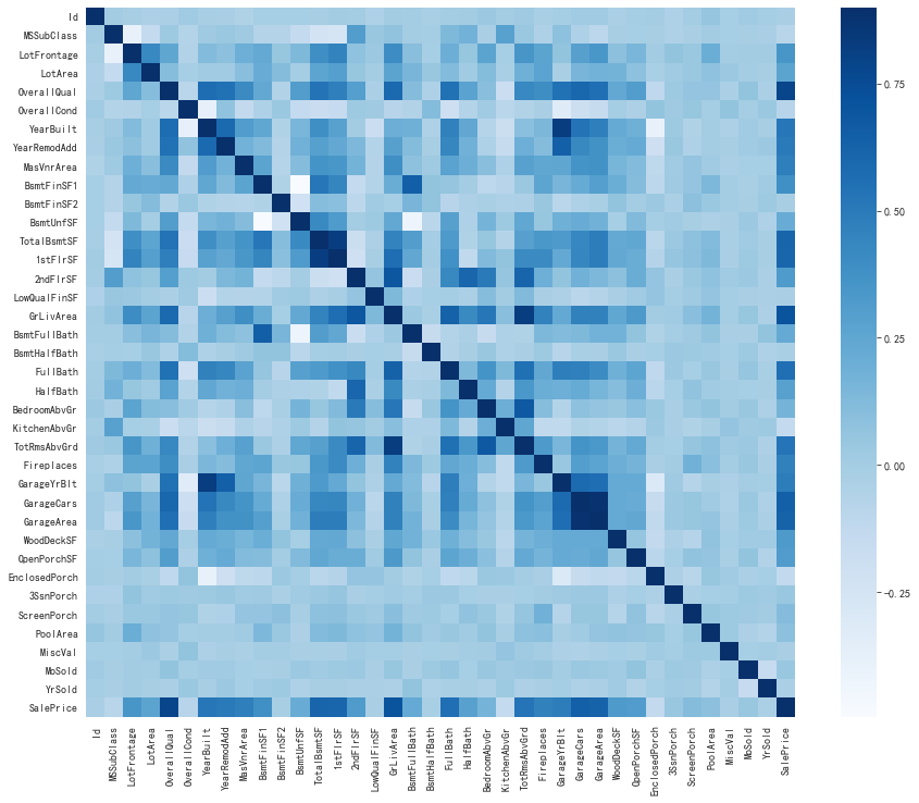
#查看它们与销售价格之间的关系
corr=train.corr()
plt.subplots(figsize=(15,12))
sns.heatmap(corr,vmax=0.9,cmap='Blues',square=True)
#查看OverallQual(综合素质)和销售价格的关系
data=pd.concat([train['SalePrice'],train['OverallQual']],axis=1)
f,ax=plt.subplots(figsize=(8,6))
fig=sns.boxplot(x=train['OverallQual'],y=train['SalePrice'],data=data)
fig.axis(ymin=0,ymax=800000)
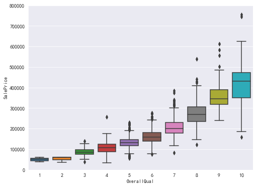
可以看出,OverallQual20000的为异常值;
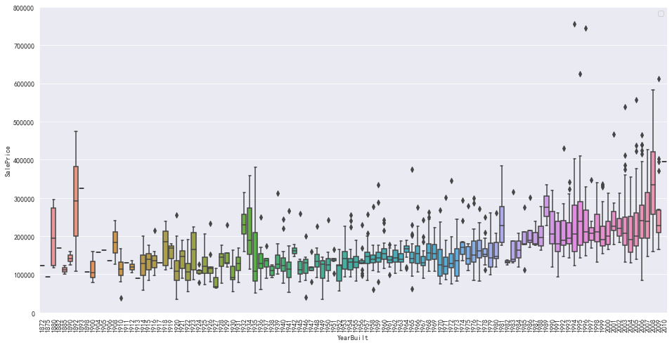
#查看YearBuilt(建筑年度)和销售价格的关系
data=pd.concat([train['SalePrice'],train['YearBuilt']],axis=1)
f,ax=plt.subplots(figsize=(16,8))
fig=sns.boxplot(x=train['YearBuilt'],y=train['SalePrice'],data=data)
fig.axis(ymin=0,ymax=800000)
plt.xticks(rotation=90)
plt.legend()
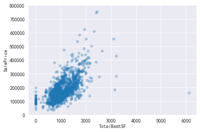
#查看TotalBsmtSF和销售价格的关系
data=pd.concat([train['SalePrice'],train['TotalBsmtSF']],axis=1)
data.plot.scatter(x='TotalBsmtSF',y='SalePrice',alpha=.3,ylim=(0,800000))
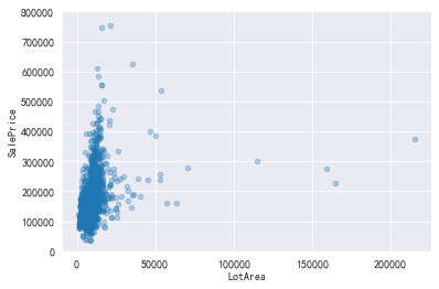
#查看LotArea和销售价格的关系
data=pd.concat([train['SalePrice'],train['LotArea']],axis=1)
data.plot.scatter(x='LotArea',y='SalePrice',alpha=.3,ylim=(0,800000))
#查看GrLivArea和销售价格的关系
data=pd.concat([train['SalePrice'],train['GrLivArea']],axis=1)
data.plot.scatter(x='GrLivArea',y='SalePrice',alpha=.3,ylim=(0,800000))
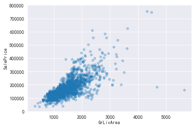
可以看出,GrLivArea>4500 and SalePrice<300000的是异常值
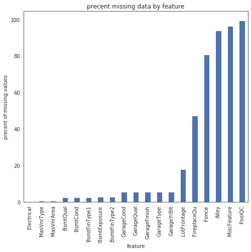
#数据缺失程度
sns.set_style("white")
f,ax=plt.subplots(figsize=(8,7))
sns.set_color_codes(palette='deep')
missing=round(train.isnull().mean()*100,2)
missing=missing[missing>0]
missing.sort_values(inplace=True)
missing.plot.bar(color='b')
plt.ylabel('precent of missing values')
plt.xlabel('feature')
plt.title("precent missing data by feature")
3 特征工程
3.1 标签转换
sns.distplot(train['SalePrice'],color='b')
plt.ylabel("frequency")
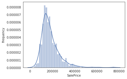
#可知SalePrice的分布是有偏的,非正态分布,大多数模型都很难处理,因此需要转换成正态分布
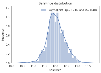
#通过对数log1p变换,转成正态分布
train['SalePrice']=np.log1p(train['SalePrice'])

#获取新分布的均值和方差
(mu,sigma)=norm.fit(train['SalePrice'])
print((mu,sigma))
(12.024057394918406, 0.39931245219387496)
sns.distplot(train['SalePrice'],color='b')
plt.legend(["Normal dist. ($\mu=${:0.2f} and $\sigma=${:0.2f})".format(mu,sigma)],loc='best')
plt.title("SalePrice distribution")
plt.ylabel("frequency")
3.2 剔除异常值
train.drop(train[(train['OverallQual']<5) & (train['SalePrice']>200000)].index,inplace=True)
train.drop(train[(train['GrLivArea']>4500) & (train['SalePrice']<300000)].index,inplace=True)
train.reset_index(drop=True,inplace=True)

train_label=train['SalePrice'].reset_index(drop=True)
train_features=train.drop(['SalePrice'],axis=1)
test_features=test

#把所有的特征合并,进行统一处理
all_features=pd.concat([train_features,test_features]).reset_index(drop=True)
all_features.drop(['Id'],axis=1,inplace=True)
all_features.shape
3.3 填补缺失值
3.3.1 类别型
#有些特征有数值型,需要都转变成str
all_features['MSSubClass']=all_features['MSSubClass'].apply(str)
all_features['YrSold']=all_features['YrSold'].apply(str)
all_features['MoSold']=all_features['MoSold'].apply(str)
all_features['Functional'].value_counts()
Typ     2715
Min2      70
Min1      65
Mod       35
Maj1      19
Maj2       9
Sev        2
Name: Functional, dtype: int64
#把Functional的缺失值用它的众数填充
all_features['Functional']=all_features['Functional'].fillna('Typ')

all_features['Functional'].mode()[0]

all_features['Electrical']=all_features['Electrical'].fillna(all_features['Electrical'].mode()[0])

all_features['KitchenQual']=all_features['KitchenQual'].fillna(all_features['KitchenQual'].mode()[0])

all_features['Exterior1st']=all_features['Exterior1st'].fillna(all_features['Exterior1st'].mode()[0])

all_features['Exterior2nd']=all_features['Exterior2nd'].fillna(all_features['Exterior2nd'].mode()[0])

all_features['SaleType']=all_features['SaleType'].fillna(all_features['SaleType'].mode()[0])

#不同MSSubClass下MSZoning的值的个数不一样,因此先按照MSSubClass进行聚合再去众数
all_features.groupby("MSSubClass")["MSZoning"].value_counts()
all_features['MSZoning']=all_features.groupby("MSSubClass")["MSZoning"].transform(lambda x:x.fillna(x.mode()[0]))

#对于NaN值通过NNone进行填充
all_features['PoolQC']=all_features['PoolQC'].fillna("None")
#对于garage(车库)相关的特征用0填充
for col in ['GarageYrBlt','GarageArea','GarageCars']:
    all_features[col]=all_features[col].fillna(0)

#对于basement(地下室)缺失就是没有
for col in ['BsmtQual','BsmtCond','BsmtExposure','BsmtFinType1','BsmtFinType2']:
    all_features[col]=all_features[col].fillna('None')

# lot Frontages(很多正面),从neighborhood的分组中去中值
all_features['LotFrontage']=all_features.groupby("Neighborhood")["LotFrontage"].transform(lambda x:x.fillna(x.mode()[0]))

# 对于其他的,都统一填充成None
obj=[]
for i in all_features.columns:
    if all_features[i].dtype==object:
        obj.append(i)
all_features.update(all_features[obj].fillna('None'))
3.3.2 数值型
#所有数值型特征
num_dtypes=['int16','int32','int64','float16','float32','float64']
not_plot=['Id']
num=[]
for i in all_features.columns:
    if all_features[i].dtypes in num_dtypes:
        if i in not_plot: pass
        else:num.append(i)

#全部填充为0
all_features.update(all_features[num].fillna(0))
3.3.3 最后检查
#数据缺失程度
missing=round(all_features.isnull().mean()*100,2)
missing=missing[missing>0]
missing.sort_values(inplace=True)
missing
3.4 解决斜率特征
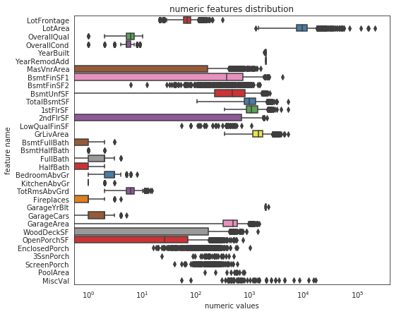
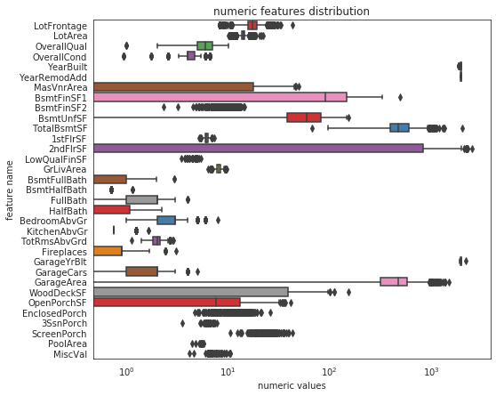
#所有数值型特征
num_dtypes=['int16','int32','int64','float16','float32','float64']
not_plot=['Id']
num=[]
for i in all_features.columns:
    if all_features[i].dtypes in num_dtypes:
        if i in not_plot: pass
        else:num.append(i)

#通过box plot查看所有数值型特征
sns.set_style("white")
f,ax=plt.subplots(figsize=(8,7))
ax.set_xscale("log")
ax=sns.boxplot(data=all_features[num],orient='h',palette='Set1')
ax.xaxis.grid(False)
plt.ylabel("feature name")
plt.xlabel("numeric values")
plt.title("numeric features distribution")
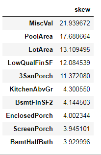
#查看所有数值型特征的偏度
skew_features=all_features[num].apply(lambda x:skew(x)).sort_values(ascending=False)

#筛选出高偏度的
high_skew=skew_features[skew_features>0.5]
skew_index=high_skew.index

#把这些高偏度给打印出来
skewness=pd.DataFrame({'skew':high_skew})
skewness.head(10)
Box-Cox 变换是常见的一种数据变换,用 于连续的响应变量不满足正态分布的情况。Box-Cox变换之后,可以一定程度上减小不可观测的误差和预测变量的相关性。比如在使用线性回归的时候,由于残差 epsilon 不符合正态分布而不满足建模的条件,这时候要对响应变量Y进行变换,把数据变成正态的。
这是一种根据数据自动寻找「最佳」变换函数的方法
#通过scipy函数的boxcox1p来进行box-cox转换,目标是找到一个简单的转换方式使得数据规范化
for i in skew_index:
    all_features[i]=boxcox1p(all_features[i],boxcox_normmax(all_features[i]+1))

#再查看变换后的分布
sns.set_style("white")
f,ax=plt.subplots(figsize=(8,7))
ax.set_xscale("log")
ax=sns.boxplot(data=all_features[num],orient='h',palette='Set1')
ax.xaxis.grid(False)
plt.ylabel("feature name")
plt.xlabel("numeric values")
plt.title("numeric features distribution")
3.5 创造特征
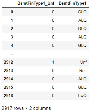
#传统的ML模型很难识别更复杂的模式,所以需要我们基于对数据集的直观理解,创建一些特征:每个房子地板的总面积、浴室和门廊面积等
all_features['BsmtFinType1_Unf']=1*(all_features['BsmtFinType1']=='Unf')

all_features[['BsmtFinType1_Unf','BsmtFinType1']]
#是否有WoodDeck(木甲板)
all_features['HasWoodDeck']=1*(all_features['WoodDeckSF']==0)

#是否有开放式门廊
all_features['HasOpenPorch']=1*(all_features['OpenPorchSF']==0)

#是否有封闭的门廊
all_features['HasEnclosedPorch']=1*(all_features['EnclosedPorch']==0)

#是否有3SsnPorch门廊
all_features['Has3SsnPorch']=1*(all_features['3SsnPorch']==0)

#是否有ScreenPorch门廊
all_features['HasScreenPorch']=1*(all_features['ScreenPorch']==0)

#重新装修的年份
all_features['YearsSinceRemodel']=all_features['YrSold'].astype(int)-all_features['YearRemodAdd'].astype(int)


#房子总的质量
all_features['Total_home_Quality']=all_features['OverallQual']+all_features['OverallCond']

#删除一些不必要的特征
all_features=all_features.drop(['Utilities','Street','PoolQC'],axis=1)

#总SF
all_features['TotalSF']=all_features['TotalBsmtSF']+all_features['1stFlrSF']+all_features['2ndFlrSF']

all_features['YrBltAndRemod']=all_features['YearBuilt']+all_features['YearRemodAdd']

all_features['Total_sqr_footage']=all_features['BsmtFinSF1']+all_features['BsmtFinSF2']+all_features['1stFlrSF']+all_features['2ndFlrSF']

all_features['Total_Bathrooms']=all_features['FullBath']+0.5*all_features['HalfBath']+all_features['BsmtFullBath']+0.5*all_features['BsmtHalfBath']

all_features['Total_porch_sf']=all_features['OpenPorchSF']+all_features['3SsnPorch']+\
                        all_features['ScreenPorch']+all_features['EnclosedPorch']+all_features['WoodDeckSF']

all_features['TotalBsmtSF']=all_features['TotalBsmtSF'].apply(lambda x:np.exp(6) if x<=0.0 else x )

all_features['2ndFlrSF']=all_features['2ndFlrSF'].apply(lambda x:np.exp(6.5) if x<=0.0 else x )

all_features['GarageArea']=all_features['GarageArea'].apply(lambda x:np.exp(6) if x<=0.0 else x)

all_features['GarageArea']=all_features['GarageArea'].apply(lambda x:np.exp(6) if x<=0.0 else x )

all_features['GarageCars']=all_features['GarageCars'].apply(lambda x:0 if x<=0.0 else x )

all_features['LotFrontage']=all_features['LotFrontage'].apply(lambda x:np.exp(4.2) if x<=0.0 else x )

all_features['MasVnrArea']=all_features['MasVnrArea'].apply(lambda x:np.exp(4) if x<=0.0 else x )

all_features['BsmtFinSF1']=all_features['BsmtFinSF1'].apply(lambda x:np.exp(6.5) if x<=0.0 else x )

all_features['haspool']=all_features['PoolArea'].apply(lambda x:1 if x>0 else x )

all_features['has2ndfloor']=all_features['2ndFlrSF'].apply(lambda x:1 if x>0 else x )

all_features['hasgarage']=all_features['GarageArea'].apply(lambda x:1 if x>0 else x )

all_features['hasbsmt']=all_features['TotalBsmtSF'].apply(lambda x:1 if x>0 else x )

all_features['hasfireplace']=all_features['Fireplaces'].apply(lambda x:1 if x>0 else x )
3.6 特征转换
#通过计算数值特征的对数平方变化来获取更多的特征

def logs(res,ls):
    m=res.shape[1]
    for i in ls:
        res=res.assign(newcol=pd.Series(np.log(1.01+res[i])).values)
        res.columns.values[m]=i+'_log'
        m+=1
    return res

log_features=['LotFrontage','LotArea','MasVnrArea','BsmtFinSF1','BsmtFinSF2','BsmtUnfSF',
             'TotalBsmtSF','1stFlrSF','2ndFlrSF','LowQualFinSF','GrLivArea','BsmtFullBath','BsmtHalfBath',
             'FullBath','HalfBath','BedroomAbvGr','KitchenAbvGr','TotRmsAbvGrd','Fireplaces','GarageCars',
              'GarageArea','WoodDeckSF','OpenPorchSF','EnclosedPorch','3SsnPorch','ScreenPorch','PoolArea',
              'MiscVal','YearRemodAdd','TotalSF']

all_features=logs(all_features,log_features)


def squares(res,ls):
    m=res.shape[1]
    for i in ls:
        res=res.assign(newcol=pd.Series(res[i]*res[i]).values)
        res.columns.values[m]=i+'_sq'
        m+=1
    return res

sq_features=['YearRemodAdd','LotFrontage_log','TotalBsmtSF_log','1stFlrSF_log','2ndFlrSF_log',
            'GrLivArea_log','GarageCars_log','GarageArea_log']


all_features=squares(all_features,sq_features)
3.7 编码分类特征
all_features=pd.get_dummies(all_features).reset_index(drop=True)
all_features.shape

#去重
all_features=all_features.loc[:,~all_features.columns.duplicated()]
4 创建训练和测试集
#重新创建训练和数据集
X=all_features.iloc[:len(train_label),:]
X_test=all_features.iloc[len(train_label):,:]

X.shape,train_label.shape,X_test.shape
((1458, 378), (1458,), (1459, 378))
4.1 可视化特征
#画出所有数值型特征
num_dtypes=['int16','int32','int64','float16','float32','float64']
not_plot=['TotalSF','Total_Bathroom','Total_porch_sf','haspool','hasgarage','hasbsmt','hasfireplace','Id']
num=[]
for i in X.columns:
    if X[i].dtypes in num_dtypes:
        if i in not_plot: pass
        else:num.append(i)

fig,axs=plt.subplots(ncols=2,nrows=0,figsize=(12,150))
plt.subplots_adjust(right=2)
plt.subplots_adjust(top=2)
sns.color_palette("husl",8)
for i,feature in  enumerate(list(X[num]),1):
    if(feature=='MiscVal'):
        break
    plt.subplot(len(list(num)),3,i)
    sns.scatterplot(x=feature,y='SalePrice',hue='SalePrice',palette='Blues',data=train)

    plt.xlabel('{c}'.format(c=feature),size=15,labelpad=12.5)
    plt.ylabel("SalePrice",size=15,labelpad=12.5)

    for j in range(2):
        plt.tick_params(axis='x',labelsize=12)
        plt.tick_params(axis='y',labelsize=12)
    plt.legend(loc='best',prop={'size':10})
plt.show()
5 模型训练
5.1 设置交叉验证和度量
kf=KFold(n_splits=12,random_state=42,shuffle=True)

def rmsle(y,y_pred):
    return np.sqrt(mean_squared_error(y,y_pred))

def cv_rmse(model,X=X):
    rmse=np.sqrt(-cross_val_score(model,X,train_label,scoring="neg_mean_squared_error",cv=kf))
    return (rmse)
5.2 设置模型
lightgbm = LGBMRegressor(objective='regression',
                       num_leaves=6,
                       learning_rate=0.01,
                       n_estimators=7000,
                       max_bin=200,
                       bagging_fraction=0.8,
                       bagging_freq=4,
                       bagging_seed=8,
                       feature_fraction=0.2,
                       feature_fraction_seed=8,
                       min_sum_hessian_in_leaf = 11,
                       verbose=-1,
                       random_state=42)

# XGBoost Regressor
xgboost = XGBRegressor(learning_rate=0.01,
                       n_estimators=6000,
                       max_depth=4,
                       min_child_weight=0,
                       gamma=0.6,
                       subsample=0.7,
                       colsample_bytree=0.7,
                       objective='reg:linear',
                       nthread=-1,
                       scale_pos_weight=1,
                       seed=27,
                       reg_alpha=0.00006,
                       random_state=42)

# Ridge Regressor
ridge_alphas = [1e-15, 1e-10, 1e-8, 9e-4, 7e-4, 5e-4, 3e-4, 1e-4, 1e-3, 5e-2, 1e-2, 0.1, 0.3, 1, 3, 5, 10, 15, 18, 20, 30, 50, 75, 100]
ridge = make_pipeline(RobustScaler(), RidgeCV(alphas=ridge_alphas, cv=kf))

# Support Vector Regressor
svr = make_pipeline(RobustScaler(), SVR(C= 20, epsilon= 0.008, gamma=0.0003))

# Gradient Boosting Regressor
gbr = GradientBoostingRegressor(n_estimators=6000,
                                learning_rate=0.01,
                                max_depth=4,
                                max_features='sqrt',
                                min_samples_leaf=15,
                                min_samples_split=10,
                                loss='huber',
                                random_state=42)

# Random Forest Regressor
rf = RandomForestRegressor(n_estimators=1200,
                          max_depth=15,
                          min_samples_split=5,
                          min_samples_leaf=5,
                          max_features=None,
                          oob_score=True,
                          random_state=42)

# Stack up all the models above, optimized using xgboost
stack_gen = StackingCVRegressor(regressors=(xgboost, lightgbm, svr, ridge, gbr, rf),
                                meta_regressor=xgboost,
                                use_features_in_secondary=True)

#use_features_in_secondary:bool(默认值:False)  --其实就是基分类器是否使用原先的特征作为输入。
#如果为True,元分类器(基分类器、meta_regressor)将根据原始回归器和原始数据集的预测进行训练。
#如果是False,则元回归器将仅接受原始回归者的预测训练。

#https://www.cnblogs.com/Christina-Notebook/p/10063146.html
5.3 训练
5.3.1 单模型
#lgb
scores={}
score=cv_rmse(lightgbm)

print("lgb:{:0.4f}({:0.4f})".format(score.mean(),score.std()))
scores['lgb']=(score.mean(),score.std())

#xgb
score=cv_rmse(xgboost)
print("xgb:{:0.4f}({:0.4f})".format(score.mean(),score.std()))
scores['xgb']=(score.mean(),score.std())

#svr
score=cv_rmse(svr)
print("svr:{:0.4f}({:0.4f})".format(score.mean(),score.std()))
scores['svr']=(score.mean(),score.std())

#ridge
score=cv_rmse(ridge)
print("ridge:{:0.4f}({:0.4f})".format(score.mean(),score.std()))
scores['ridge']=(score.mean(),score.std())

#rf
score=cv_rmse(rf)
print("rf:{:0.4f}({:0.4f})".format(score.mean(),score.std()))
scores['rf']=(score.mean(),score.std())

#gbr
score=cv_rmse(gbr)
print("gbr:{:0.4f}({:0.4f})".format(score.mean(),score.std()))
scores['gbr']=(score.mean(),score.std())
lgb:0.1165(0.0165)
xgb:0.1363(0.0167)
svr:0.1093(0.0200)
ridge:0.1101(0.0161)
rf:0.1367(0.0188)
gbr:0.1122(0.0166)
5.3.2 混合模型
为了防止过拟合和模型更加鲁棒
ridge_model_full_data=ridge.fit(X,train_label)
svr_model_full_data=svr.fit(X,train_label)
gbr_model_full_data=gbr.fit(X,train_label)
xbg_model_full_data=xgboost.fit(X,train_label)
lgb_model_full_data=lightgbm.fit(X,train_label)
rf_model_full_data=rf.fit(X,train_label)
stack_gen_model=stack_gen.fit(np.array(X),np.array(train_label))
def blended_predictions(X):
return ((0.1*ridge_model_full_data.predict(X))+\
(0.2*svr_model_full_data.predict(X))+\
(0.1*gbr_model_full_data.predict(X))+\
(0.1*xbg_model_full_data.predict(X))+\
(0.1*lgb_model_full_data.predict(X))+\
(0.05*rf_model_full_data.predict(X))+\
(0.35*stack_gen_model.predict((np.array(X))))
)
blended_score=rmsle(train_label,blended_predictions(X))
scores['blended']=(blended_score,0)
print('Rmsle score on train data:\ ',blended_score)
Rmsle score on train data:\ 0.07576005937888909
5.3.3 确定性能最佳的模型
sns.set_style("white")
fig=plt.figure(figsize=(24,12))

ax=sns.pointplot(x=list(scores.keys()),y=[score for score,_ in scores.values()],markers=['o'],linestyles=['-'])

for i ,score in enumerate(scores.values()):
    ax.text(i,score[0]+0.002,'{:.6f}'.format(score[0]),horizontalignment='left',size='large',color='black')

plt.ylable("Score (RMSE)",size=20)
plt.xlable("Model",size=20)
6 预测
submisson=pd.read_csv("./data/sample_submission.csv")
submisson.shape

#通过expm1反变换回去
submisson.iloc[:,1]=np.floor(np.expm1(blended_predictions(X_test)))

#去除一些异常值
q1=submisson['SalePrice'].quantile(0.0045)
q2=submisson['SalePrice'].quantile(0.99)
submisson['SalePrice']=submisson['SalePrice'].apply(lambda x:x if x>q1 else x*0.77)
submisson['SalePrice']=submisson['SalePrice'].apply(lambda x:x if x<q2 else x*1.1)

submisson.to_csv("submisson_1.csv",index=False)

 浙公网安备 33010602011771号