PID控制器(比例-积分-微分控制器)- IV
调节/测量放大电路电路图:PID控制电路图

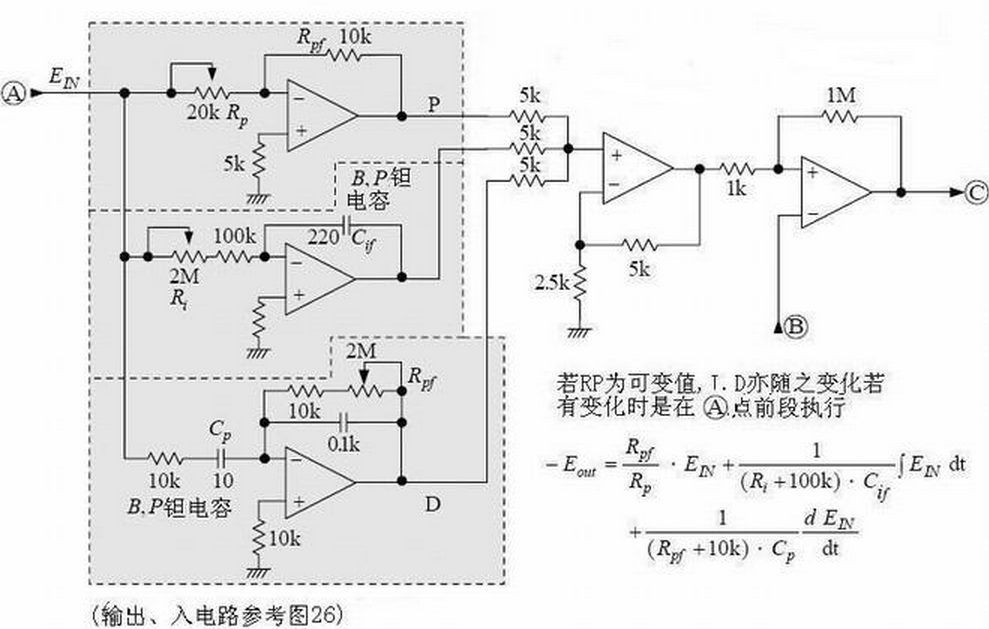
如图是PlD控制电路,即比例(P)、积分(I)、微分(D)控制电路。
A1构成的比例电路与环路增益有关,调节RP1,可使反相器的增益在0·5一∞范围内变化;
A2是积分电路,积分时间常数可在22一426S范围内变化;
A3是微分电路,时间常数由Cl(Rl+R(RP3))决定;
A4将比例、积分、微分各电路输出倒相后合成为U。
Controller Circuit
This circuit is the basis of a temperature controller.
Study it and then answer the questions that follow.
The questions have links to outline answers but please resist the temptation to look at these
until you have written down your own answers to all the questions.
- What does the circuit do and how does it work?
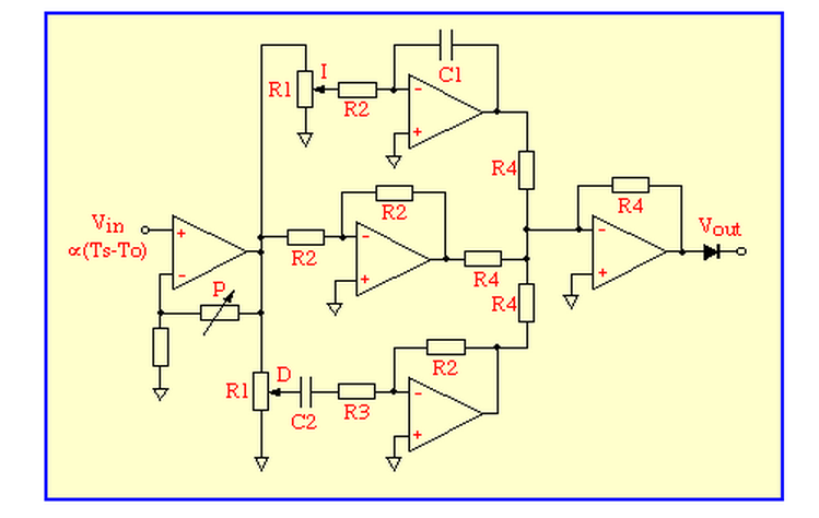
The circuit is a form of PID controller.
The input signal is buffered and amplified by a non-inverting amplifier and the gain of this stage defines the proportional gain P of the controller.
The amplified error signal passes in parallel through
an integrator (top) a unity-gain amplifier (middle) and a differentiator (bottom) all of which have inverting behaviour.
Their outputs are then summed and inverted by the final op-amp and passed to the output.
The potentiometers labelled D and I control the proportions in which derivative and integral fractions contribute
to the output signal which is proportional to the power W to be supplied to the heater. - What additional circuit is needed between the output and the heater?
A heater-driver that ensures that the power dissipated in the heater is proportional to the output voltage.
This is usually either a square-rooter if the heater is to be driven by DC, or with AC heaters some type of pulse-width modulator. - Why is there a diode in series with the output?
The heater power can only be positive or zero so the diode keeps the output signal within these constraints. - Why might one want to make R2 much larger than R1?
A low value of R2 would 'load' the potentiometers and impair the linear relationship between control position and gain. - What is the purpose of R3?
The gain of a differentiator increases in proportion to frequency and without R3 it would only be limited by the,
normally unnecessarily high, open-loop gain of the op-amp.
R3 limits the gain at high frequencies reducing the noise of the system. - What might be the most serious effect of op-amp offset voltages currents and bias?
It is most likely to be troublesome by causing an offset between the set-point and oven temperatures.
Under some circumstances the integrator may drift and eventually saturate which would prevent it from working properly. - How might the impact of op-amp offset and bias be reduced?
The first thing to try would be a resistor, equal in value to R2, between the positive input of the integrating op-amp
and ground to eliminate the common-mode bias current.
Selecting an op-amp with a good input-offset performance would be the next step. - How would you consider improving the circuit?
The improvements suggested in the previous answer would be a good start.
The diode at the output could be replaced by an active rectifier for greater precision at low heater powers.
Some method of reseting the integrator would help and maybe a circuit implement
the 'Limit I?' function of the interactive simulation.
Meters to indicate heater power and an error signal are helpful to the person who has to tune a controller for a particular oven.
PID Controller

Tuning the PID controller can be like learning to roller blade, ski or maybe riding a bull.
Until you've done it a few times, the literature you've read really doesn't hit home. But after after few attempts (and falls),
you find it wasn't so bad after all - in fact it was kind of fun!
The PID controller is every where - temperature, motion, flow controllers - and its available in analog and digital forms.
Why use it? It helps get your output (velocity, temperature, position) where you want it,
in a short time, with minimal overshoot, and with little error.
In many applications the PID controller can do the job - but as usual, with compromises.
After a short intro to the PID terms and an example control system, you'll get a chance tune a PID controller.
THE CONTROL SYSTEM
The SPICE circuit for the Control System looks pretty much like the block diagram.
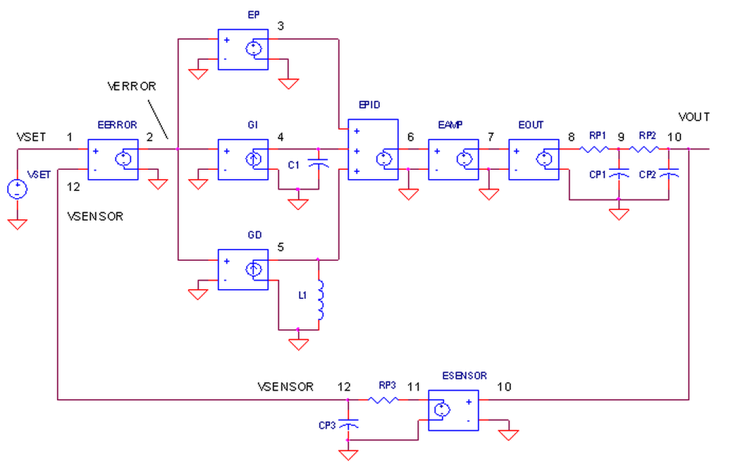
PID CONTROLLER.
How do we create the PID terms? To get theProportional term, EP multiples Verror at V(2) by a fixed gain of 1 - easy enough! To get the Integral term, current source GI converts V(2) to a current and integrates it on C1=1F. Finally, theDerivative term is created by GD converting V(2) to a current and forcing it through L1. The resulting voltage becomes V(5) = L1 di / dt. A quick substitution of L1 = 1 H and i = Verror gets you V(5) = d Verror / dt.
OUTPUT PROCESS.
EOUT represents a very simplified model of a process to be controlled like motor velocity or heater temperature. The gain of 100 could represent an output transfer function of 100 RPM / V or 100 ° C / V. To include the effects of the motor's inertia or heater's thermal mass, we've added some time delay into the output using two cascaded RC filters. Although Vout is simulated in volts, we know it really represents other variables like velocity in RPM or temperature in °C.
SENSOR.
The sensor tells you, typically by a voltage, what's happening at the control system output. For motor velocity, a tachometer could generate 1 V / 100 RPM; for temperature, a thermistor circuit could produce 0.01 V / deg C. ESENSOR models this feedback device. Because a sensor does not respond instantly, an RC filter is also added here to model its finite response time.
TUNING THE PID CONTROLLER
Although you'll find many methods and theories on tuning a PID,
here's a straight forward approach to get you up and soloing quickly.
1. SET KP. Starting with KP=0, KI=0 and KD=0, increase KP until the output starts overshooting and ringing significantly.
2. SET KD. Increase KD until the overshoot is reduced to an acceptable level.
3. SET KI. Increase KI until the final error is equal to zero.
Run a simulation of the circuit file PID1.CIR.
VSET generates a 10V step input voltage to the control system.
You can adjust the PID terms at the EPID source that adds the P, I and D terms at V(3), V(4) and V(5).
Initially, the PID multipliers are set to KP=1, KI=0 and KD=0.
EPID 6 0 POLY(3) (3,0) (4,0) (5,0) 0 1 0 0
SET KP.
Plot the system input V(1) and the sensor output (12). Although the response looks smooth, what is the sensor voltage compared to the desired 10V? The output falls short by 5V! To reduce this error, increase KP to 10 (Change EPID to look like ... 10 0 0 ). Wow, the output now reaches 9V, reducing the error to 1V. But as you can see, the output is getting wild with overshoot and ringing. Push KP up higher to 20 or 30. Yes, the error reduces, but the overshoot gets worse. Eventually, your system will become unstable and break out into song (oscillate). Back off KP to 20 or so.
SET KD.
The derivative term can rescue the response by counteracting the KP drive when the output is changing. Start with a small value like KD=0.2 and rerun the simulation (Change EPID to look like ...
20 0 0.2 ). Now you're wrestling control back into the system - the ringing and overshoot are reduced! Crank up KD some more. Improvement should continue to a point where the system becomes less stable and overshoot increases again. Return KD to around 0.5.
SET KI.
With KP=20, KI=0 and KD=0.5 the response looks respectable, but the final error is a disappointing 0.5V (or 5%)! Now, try the KI term. This will integrate the remaining error into a drive signal big enough to reduce the error further. Start with KI = 10 ( EPID should look like ... 20 10 0.5 ). Check out the last half of the V(12) - the sensor output moves slowly toward 10V! You might want to put up a cursor on the plot to monitor the exact value of V(12). The bigger you make KI, the faster it will move toward 10V. Like the other terms, a value is reached where the KI does more harm than good as the system becomes less stable.
DIVING DEEPER
Diving a little deeper you can get a clearer view of the PID components. Before we go beneath the surface, set KP=10, KI=0 and KD=0.
Run a couple of simulations with KP=10 and KP 20. Plot V(1) and V(12). What is the final error for each case? You may have noticed the errors of 1 and 0.5V are proportional to the gains of 10 and 20. You can estimate the error by
Verror ≈ Vset / KP
for large KP. What kind of gain do you need for a 1% error? You can easily calculate it as a gain of 100. However, we've already seen how large gain cause overshoot, ringing and oscillations! KP can't do it alone.
KD counteracts KP - let's see how. Set KP back to 10 and run a simulation. Plot the P function V(3) which is really Verror. Now plot the D term V(5) which we know is dVerror / dt. To get a good view of D, set the Y-Axis limits to +100 /-200V. Notice how dVerror / dt swings negative when Verror is initially positive. How does this help? Essentially D counteracts the P term potentially reducing ringing and oscillations. The nice thing about the D term is that it goes to zero as the output settles. This makes sense - no change in output, no derivative term. Add in some of the D function by setting the multipliers to KP=10, KI=0 and KD=0.5. The initial overshoot should be significantly reduced.
We've seen how a large gain produces a small error. However, big KP gets you into big trouble with overshoot and ringing. Alternatively, an integrator can also give you a big gain by accumulating even a small error over time. Run a simulation with KP=10, KI=0 and KD=0.5 and plot the I term at V(4). What does it look like? Notice, a ramp function, representing Verror integrated over over time, builds up to a significant drive voltage. Add in the I function by setting KP=10, KI=40 and KD=0.5. The I term completes the controller's job by moving the output toward an error of zero.
SIMULATION NOTE
Need a handy way to combine multiple signals such as the PID sum? A controlled source can be a function of multiple inputs described by a polynomial. What is this polynomial? The equation is defined by a coefficient list at the end of the statement. The example below
EPID 6 0 POLY(3) (3,0) (4,0) (5,0) 0 10 2 1
creates a polynomial of the form
V(6,0) = 0 + 10 ∙ V(3,0) + 2 ∙ V(4,0) + 1 ∙ V(5,0)
or more generally,
VO = k0 + k1∙V1 + k2∙V2 + k3∙V3
In fact, you can get higher order terms and cross terms by extending the coefficient list
VO = ...+ k4∙V1∙V1 + k5∙V1∙V2 + k6∙V1∙V3 +
+ k7∙V2∙V2 + k8∙V2∙V3 +
+ k9∙V3∙V3
If you're not using a term, you need to put a 0 in its place; you can't just leave it out.
This feature is great for simpler polynomials. Keeping track of the coefficient list for large polynomials can get crazy fast.
We've all heard about the wonders of the PID controller, bringing a system's output
- temperature, velocity, light - to its desired set point quickly and accurately.
But now, your boss says okay, design one for us.
Although there's a number of ways to do it, the circuit above nicely separates the three terms into three individual op amp circuits.
We'll build it in SPICE, test each term and finally place it inside a motor speed controller for you to tune.
If you wish, take a quick review ofPID Control.
THE PID CONTROLLER
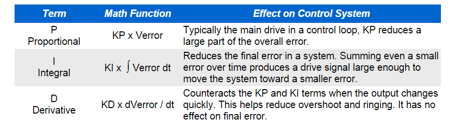
You've probably seen the terms defined before:
P -Proportional, I - Integral, D - Derivative.
These terms describe three basic mathematical functions applied to the error signal ,
Verror = Vset - Vsensor.
This error represents the difference between where you want to go (Vset), and where you're actually at (Vsensor).
The controller performs the PID mathematical functions on the error and applies the their sum to a process (motor, heater, etc.)
So simple, yet so powerful! If tuned correctly, the signal Vsensor should move closer to Vset.
Tuning a system means adjusting three multipliers Kp, Ki and Kd adding in various amounts of these functions
to get the system to behave the way you want.
The table below summarizes the PID terms and their effect on a control system.
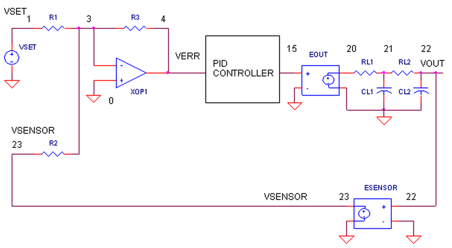
THE PID CONTROLLER
What basic components are needed for a servo system?
Many look similar to the circuit below. The error amp gives you a constant reality check.
How? It compares where you want to go, Vset, with where you're at now, Vsensor,
by calculating the difference between the two, Verr = Vset - Vsensor.
The PID controller takes this error and determines the drive voltage applied
to the process in an attempt to bring Vset = Vsensor or Verr = 0.
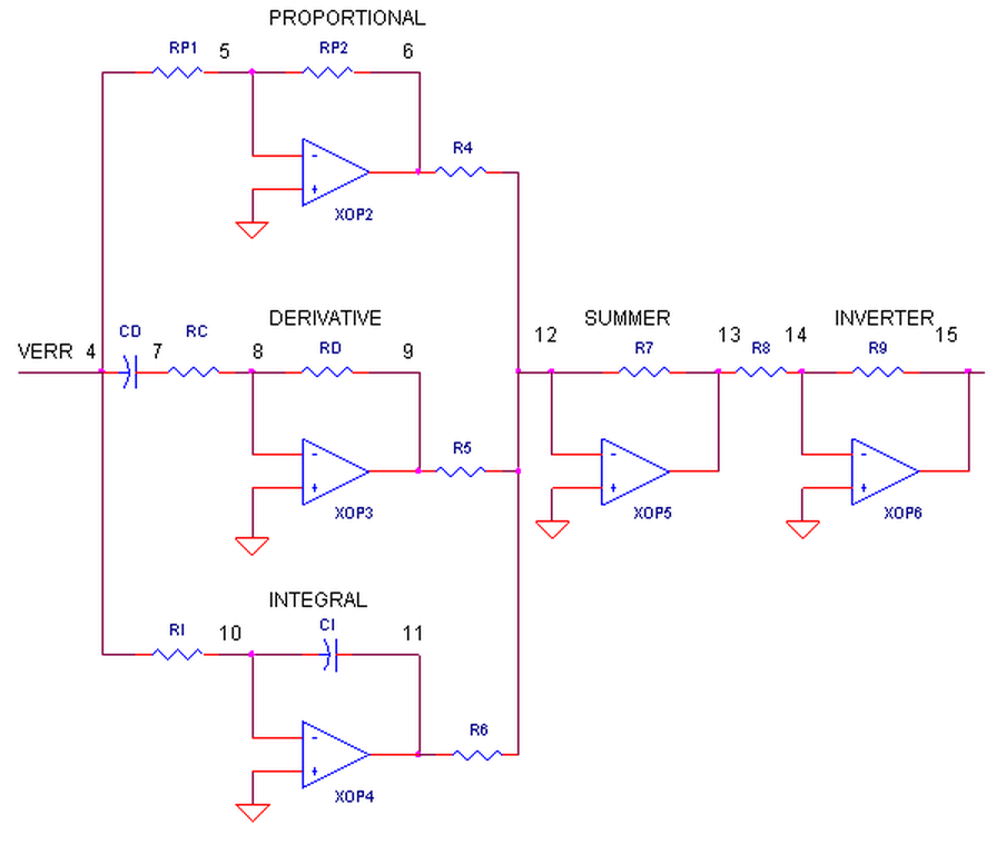
ERROR AMPLIFIER. A classic circuit for calculating the error is a summing op amp.
In the controller, XOP1 performs the error calculation. Remembering that the summing amp is an inverting amp,
we calculate its output using R1 = R2 = R3 = 10 kΩ.
Verr = - (Vset / R1 + Vsensor / R2) ∙ R3 = (Vset + Vsensor) ∙ (10 k / 10 k) = - ( Vset + Vsensor )
But how does the summer calculate a difference?
Well, it does require that your sensor circuit produce a negative output voltage.
Assuming that Vsensor is the negative of the actual sensor voltage Vsensor = - Vsens, you get the difference.
Verr = -( Vset - Vsens )
You can look at the error amp's function this way. When Vsensor is exactly the negative ofVset, the currents through R1 and R2,
equal and opposite, cancel each other as they enter the op amps's summing junction.
You end up with zero current through R3 and of course 0V, or zero error, at the output.
Any difference between Vset and -Vsensor, results in an error voltage at the output that the PID controller can act upon.
OP AMP PID CONTROLLER.
How do we get the PID terms from the error voltage Verr?
We enlist three simple op amp circuits.
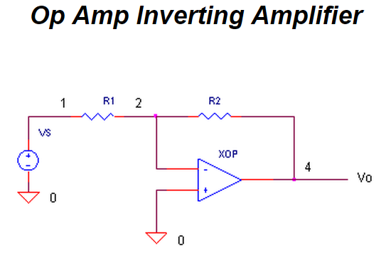
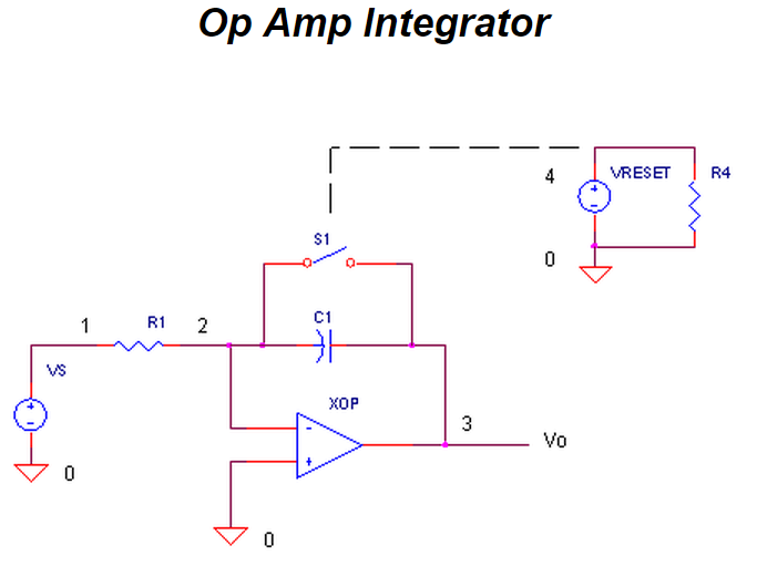
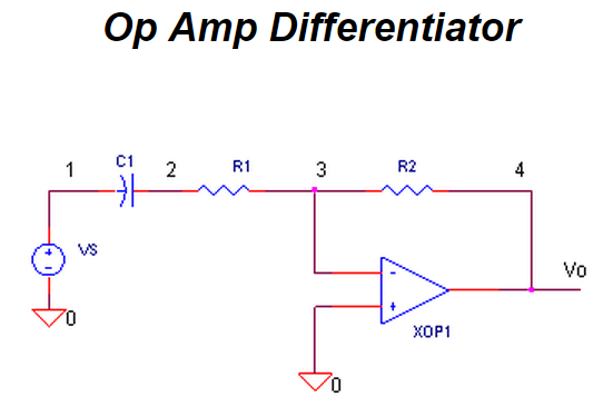
If you need, take a review of the op amp amplifier,integrator and differentiator circuits.

Lastly, we need to add the three PID terms together. Again the summing amplifier XOP5 serves us well.
Because the error amp, PID and summing circuits are inverting types,
we need to add a final op amp inverter XOP6 to make the final output positive, given a positive Vset.
OUTPUT PROCESS.
EOUT represents a very simplified model of a process to be controlled, such as motor velocity for example.
The gain of 100 could represent an output transfer function of 100 RPM / V.
To include the effects of the motor's inertia, we've added some time delay into the output using two cascaded RC filters.
Although Vout is simulated in volts, we know it really represents RPM.
SENSOR.
The sensor tells you the actual velocity at the motor, 1 V / 100 RPM for this tachometer.
ESENSOR models this feedback device. Note, this sensor block actually produces a negative output voltage,
the proper input polarity for your error amplifier as mentioned above.

 浙公网安备 33010602011771号