PID控制器（比例-积分-微分控制器）- III

PID Controller Algorithms

Controller manufacturers arrange the Proportional, Integral and Derivative modes into three different controller algorithms or controller structures.  These are called Interactive, Noninteractive, and Parallel algorithms.  Some controller manufacturers allow you to choose between different controller algorithms as a configuration option in the controller software.

Interactive Algorithm

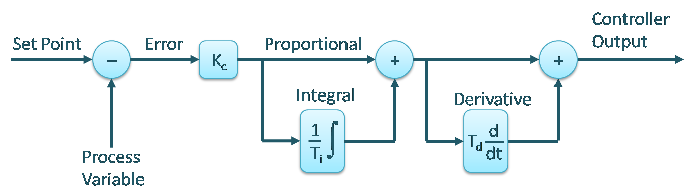
The oldest controller algorithm is called the Series, Classical, Real or Interactive algorithm.  The original pneumatic and electronic controllers had this algorithm and it is still found it in many controllers today.  The Ziegler-Nichols PID tuning rules were developed for this controller algorithm.

Noninteractive Algorithm

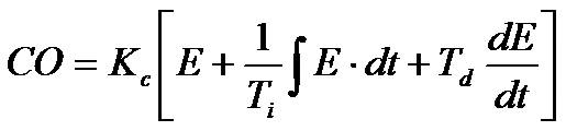
The Noninteractive algorithm is also called the Ideal, Standard or ISA algorithm. The Cohen-Coon and Lambda PID tuning rules were designed for this algorithm.

Note: If no derivative is used (i.e. T_d = 0), the interactive and noninteractive controller algorithms are identical.

Parallel Algorithm

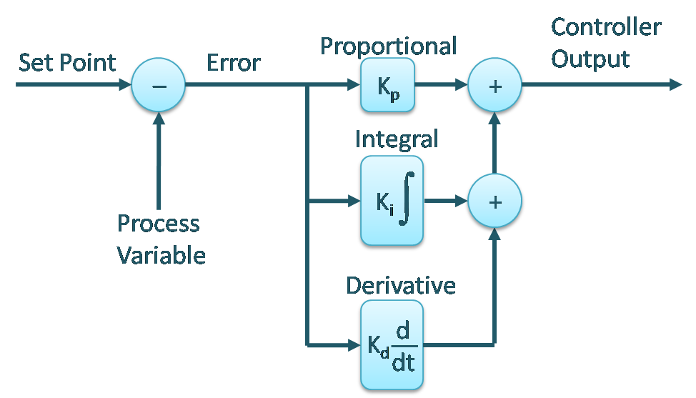
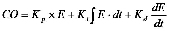
Some academic textbooks discuss the parallel form of PID controller, but it is also used in some DCSs and PLCs.  This algorithm is simple to understand, but not intuitive to tune.  The reason is that it has no controller gain (affecting all three control modes), it has a proportional gain instead (affecting only the proportional mode).  Adjusting the proportional gain should be supplemented by adjusting the integral and derivative settings at the same time.  Try to not use this controller algorithm if possible (in some DCSs it is an option, so select the alternative).

Significance of Different Algorithms

The biggest difference between the controller algorithms is that the Parallel controller has a true Proportional Gain (Kp), while the other two algorithms have a Controller Gain (Kc). Controller Gain affects all three modes (Proportional, Integral and Derivative) of the Series and Ideal controllers, while Proportional Gain affects only the Proportional mode of a Parallel controller.

This difference has a major impact on the tuning of the controllers. All the popular tuning rules (Ziegler-Nichols, Cohen-Coon, Lambda, and others) assume the controller does not have a parallel structure and therefore has a Controller Gain. To tune a Parallel controller using any of these rules, the Integral time has to be divided and derivative time multiplied by the calculated Controller Gain.

The second difference between the controller algorithms is the interaction between the Integral and Derivative modes of the Series (Interactive) controller. This, of course, is only of significance if the Derivative mode is used. In most PID controller applications, Derivative mode is not used. Formulas have been developed for converting tuning settings between Ideal and Series controller algorithms.

Units of Measure of Tuning Settings

Another very important difference between controllers lies in the units of measure of the tuning settings. There are three differences.

1. Most controller types (e.g. Honeywell Experion, Emerson DeltaV, ABB Bailey) use Controller Gain, while some (e.g. Foxboro I/A, Yokogawa CS3000) use Proportional Band (PB). The conversion between the two is easy once you know which one is being used: PB = 100% / Kc.

2. Many controllers (e.g. Siemens APACS) use minutes as the unit for Integral and Derivative modes, but some controllers (e.g. Emerson DeltaV) use seconds.

3. Some controllers (e.g. ABB Mod 300) use Time for their Integral unit, while others (e.g. Allen-Bradley SLC500) use Repeats/Time. These are reciprocals of each other.

The first controller I ever tried to tune used Proportional Band, but at the time, I had never heard of this concept. Needless to say, when I entered my calculated Kc of 1.2 into its PB setting, the loop became wildly unstable.  It did not take me long to realize that I should read up on PID controllers before trying to tune one again.

Other Differences

Beyond the differences mentioned above, controllers also differ in the way the changes on controller output is calculated (positional and velocity algorithms), in the way Proportional and Derivative modes act on set point changes, in the way the Derivative mode is limited/filtered, as well as a interesting array of other minor differences. These differences are normally subtle, and should not affect your tuning.

When tuning controllers, always find out what structure the controller has and what units it is using.

Ziegler-Nichols Closed-Loop Tuning Method

J.G. Ziegler and N.B. Nichols published two tuning methods for PID controllers in 1942.

This article describes in detail how to apply one of the two methods, sometimes called the Ultimate Cycling method. (The other one is called the process reaction-curve method.) I have seen many cryptic versions of this procedure, but they leave a lot open for interpretation, and a practitioner may run into difficulties using one of these abbreviated procedures.

Before we get started, here are a few very important notes:

• Read the entire procedure before beginning.
• This tuning method does not work for inherently unstable processes like temperature control of exothermic reactions.
• This procedure cannot be used if the Process Variable oscillates when the controller is in Manual control mode. If the loop is already oscillating in Auto, make sure the cycling stops in Manual.
• If the controller drives a control valve or damper, and this device has dead band or stiction problems, this tuning method cannot be used and will lead to inaccurate results and poor tuning at best.
• Care should be taken to always keep the process in a safe operating region.
• An experienced operator should oversee the entire test and must have the authority to terminate the test at any time.
• Keep note of the original controller settings and leave them with the operator in case he/she needs to revert back to them later. Process conditions can change significantly, and your new tuning settings might only work for the conditions at which the process tests were done.

The steps below apply to a controller with a Controller Gain setting. If your controller uses Proportional Band instead, do the reciprocal of any Controller Gain changes. E.g. if the procedure calls for increasing the Controller Gain by 50%, the Proportional Band should be decreased by 50%, etc.

To apply the Ziegler-Nichols Closed-Loop method for tuning controllers, follow these steps:

1. Stabilize the process. Make sure no process changes (e.g. product changes, grade changes, load changes) are scheduled.
2. If the loop is currently oscillating, make sure that the Process Variable stops oscillating when the controller is placed in Manual mode.
3. Remove Integral action from controller.
   • If your controller uses Integral Time (Minutes or Seconds per Repeat), set the Integral parameter to a very large number (e.g. 9999) to effectively turn it off.
   • If your controller uses Integral Gain (Repeats per Minute or Repeats per Second), set the Integral parameter to Zero.
4. Remove Derivative action by setting the Derivative parameter to Zero.
5. Place the controller in Automatic control mode if it is in Manual mode.
6. Make a Set Point change and monitor the result.
7. If the Process Variable does not oscillate at all, double the Controller Gain.
8. If the Process Variable oscillates and the amplitude of the peaks decreases, increase the Controller Gain by 50% (or less if you are getting close to a constant amplitude).
9. If the Process Variable oscillates and the amplitude of the peaks increases, decrease the controller gain by 50% (or less if you are getting close to a constant amplitude).
10. If the Process Variable or Controller Output hits its upper or lower limits, decrease the controller gain by 50%. The Process Variable and Controller Output must oscillate freely for this method to work.
11. If the oscillations have died out, go to Step 6.
12. If the loop is oscillating, but not with a constant amplitude, repeat Steps 8, 9, and 10 until oscillations with a constant amplitude are obtained.
13. If the Process Variable is oscillating with constant amplitude, and neither the Process Variable nor the Controller Output hits its limits, do the following:
    • Take note of the “Ultimate” Controller Gain (K_u). If your controller has Proportional Band, note down the “Ultimate Band” (PB_u).
    • Measure the period of the oscillation (t_u). If your controller’s Integral and Derivative units are in minutes, measure tu in minutes. It the controller uses seconds, measure t_u in seconds.
14. Cut the Controller Gain in half to let the control loop stabilize while you do the calculations.
15. Calculate new controller settings using the equations below, enter them into the controller, and make a Set Point change to test them.

The Ziegler-Nichols tuning rules were designed for a ¼ amplitude decay response. This results in a loop that overshoots its set point after a disturbance or set point change. The response in general is somewhat oscillatory, the loop is only marginally robust and it can withstand only small changes process conditions. I recommend using slightly different settings (also shown below) to obtain a robust loop with increased stability.

 

Rules for a PI Controller

The PI tuning rule can be used on controllers with interactive or noninteractive algorithms.

Controller Gain (Kc)

• Ziegler-Nichols Rule: Kc = 0.45 K_u
• For robust control use: Kc = 0.22 K_u

Proportional Band (PB)

• Ziegler-Nichols Rule: PB = 2.2 PB_u
• For robust control use: PB = 4.4 PB_u

Integral Time in Minutes per Repeat or Seconds per Repeat

• Ziegler-Nichols Rule: Ti = 0.83 t_u
• For level control (integrating processes) use: Ti = 1.6 t_u

Integral Gain in Repeats per Minutes or Repeats per Seconds

• Ziegler-Nichols Rule: Ki = 1.2 / t_u
• For level control (integrating processes) use: Ki = 0.6 / t_u

 

Rules for a PID Controller

The PID tuning rule was designed for  a controller with the Interactive algorithm. 

The tuning settings should be converted for use on controllers with Noninteractive and Parallel algorithms.

Controller Gain (Kc)

• Ziegler-Nichols Rule: Kc = 0.6 K_u
• For robust control use: Kc = 0.3 K_u

Proportional Band (PB)

• Ziegler-Nichols Rule: PB = 1.7 PB_u
• For robust control use: PB = 3.3 PB_u

Integral Time in Minutes per Repeat or Seconds per Repeat

• Ziegler-Nichols Rule: Ti = 0.5 t_u
• For level control (integrating processes) use: Ti = 1.0 t_u

Integral Gain in Repeats per Minutes or Repeats per Seconds

• Ziegler-Nichols Rule: Ki = 2.0 / t_u
• For level control (integrating processes) use: Ki = 1.0 / t_u

Derivative Time or Derivative Gain

• Td or Kd = 0.125 x t_u

For PI control, no conversion is needed.
For PID control, to convert from interactive controller parameters to noninteractive:
Set the controller gain to Kc x (Ti + Td) / Ti
Set the integral time to Ti + Td
Set the derivative time to Ti x Td / (Ti + Td).

To convert from noninteractive controller parameters to parallel:
Set proportional gain (Kp) to Kc.
Set integral gain (Ki) to Kc/Ti, or for integral time (Ti) use Ti/Kc.
Set derivative gain (Kd) to Kc x Td.

Ku is the controller gain that gives you the ultimate cycle.

You determine it experimentally through trial and error as described above.

If the cycle amplitude increases, reduce the controller gain.

If the amplitude decreases, increase the controller gain.

If the amplitude remains constant, then controller gain = Ku.

Derivative Control Explained

When doing on-site services or training, I am often asked:

When should one use the derivative control mode of a PID controller?

Although there is no black & white division between when to use it or not,

I have a few guidelines that should help your decision.

But let’s take a step back first and review the derivative control mode and its role in a PID controller.

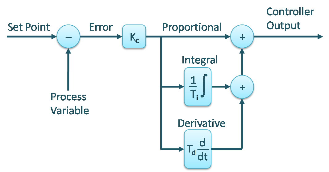
Figure 1. PID Controller

What is Derivative?

You can think of derivative control as a crude prediction of the error in future, based on the current slope of the error. How far into the future? That’s what the derivative time (Td) is for. It is the prediction horizon. (Derivative control actually uses extrapolation, not prediction. But hey, we all understand how prediction works, so I’ll just go with that.) Once the derivative mode has predicted the future error, it adds an additional control action equal to Controller Gain * Future Error.

For example, if the error changes at a rate of 2% per minute, and the derivative time Td = 3 minutes, the predicted error is 6%. If the Controller Gain, Kc = 0.2, then the derivative control mode will add an additional 0.2 * 6% = 1.2% to the controller output.

You don’t Absolutely Need Derivative
The first point to consider when thinking about using derivative is that a PID control loop will work just fine without the derivative control mode. In fact, the overwhelming majority of control loops in industry use only the proportional and integral control modes. Proportional gives the control loop an immediate response to an error, and the integral mode eliminates the error in the longer term. Hence – no derivative is needed.

Why Use Derivative
The derivative control mode gives a controller additional control action when the error changes consistently. It also makes the loop more stable (up to a point) which allows using a higher controller gain and a faster integral (shorter integral time or higher integral gain).

These have the effect of reducing the maximum deviation of process variable from set point if the process receives and external disturbance. For a typical temperature control loop, you can expect a 20% reduction in the maximum deviation. Figure 2 shows how a loop with derivative (PID) control recovers quicker from a disturbance with less deviation than a loop with P or PI control.

Figure 2. P versus PI versus PID control.

Obviously you don’t want to use derivative to speed up a loop if the control objective is slow response, like a surge tank, for example. But for loops where fast response is the objective, derivative could help. But do read on for information on when not to use derivative.

Noisy PV
Using the derivative control mode is a bad idea when the process variable (PV) has a lot of noise on it. ‘Noise’ is small, random, rapid changes in the PV, and consequently rapid changes in the error. Because the derivative mode extrapolates the current slope of the error, it is highly affected by noise (Figure 3). You could try to filter the PV so you can use derivative, as long as your filter time constant is shorter than 1/5 of your derivative time.

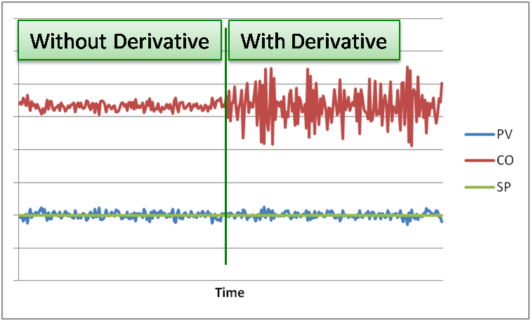
Figure 3. Effect of Noise on Derivative.

Process Dynamics
On dead-time dominant processes, PID control does not always work better than PI control (it depends on which tuning method you use). 

If the time constant (tau) is equal to or longer than the dead time (td), like in Figure 4, PID control easily outperforms PI control.

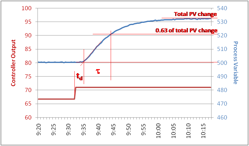
Figure 4. Process Dynamics.

Temperature and Level Loops
Temperature control loops normally have smooth measurements and long time constants. The process variable of a temperature loop tends to move in the same direction for a long time, so its slope can be used for predicting future error. So temperature loops are ideal candidates for using derivative control – if needed. Level measurements can be very noisy on boiling liquids or gas separation processes. However, if the level measurement is smooth, level control loops also lend themselves very well to using derivative control (except for surge tanks and averaging level control where you don’t need the speed).

Flow Control Loops
Flow control loops tend to have noisy PVs (depending on the flow measurement technology used). They also tend to have short time constants. And they normally act quite fast already, so speed is not an issue. These factors all make flow control loops poor candidates for using derivative control.

Pressure Control Loops
Pressure control loops come in two flavors: liquid and gas. Liquid pressure behaves very much like flow loops, so derivative should not be used. Gas pressure loops behave more like temperature loops (some even behave like level loops / integrating processes), making them good candidates for using derivative control.

Final Words
Derivative control adds another dimension of complexity to control loops. It does have its benefits, but only in special cases. If a loop does not absolutely need derivative control, don’t bother with it. However, if you have a lag-dominant loop with a smooth process variable that needs every bit of speed it can get, go for the derivative.

To learn more about controllers and tuning, contact OptiControls to for on-site process control training.

Process Control for Practitioners* - How to Tune PID controllers and Optimize Control Loops, is authored by OptiControls' principal consultant, Dr. Jacques F. Smuts, and published by OptiControls.

Control loop optimization is not rocket science, but it is not trivial either. To be effective in optimizing the performance industrial process control systems, you have to know the process and its limitations, understand process dynamics, controllers and tuning, use the right techniques and tools, and follow the optimization process systematically. You also have to know how to troubleshoot control problems to find and fix their causes.

This book conveys the knowledge and techniques required to effectively improve the performance of automatic control systems. It clearly and concisely covers all the topics and know-how required for being an outstanding controls practitioner. Explanations go into enough depth to make the material understandable, but discussions are kept short so the book can serve as a reference guide.

The book shows you how to tune PID controllers more effectively in less time, and ensure long-term loop stability. It is your complete reference for improving control-loop performance, solving process control problems, and designing control strategies. You will refer to this guide again and again.

The book's 315 pages and 176 figures will help you to:

• Understand PID controllers, their control actions, settings, and options.
• Identify process dynamics and their effects on loop performance and controller tuning.
• Get the best possible performance from a control loop.
• Tune controllers differently to achieve specific control objectives.
• Identify the root cause (or causes) of poor control performance.
• Use techniques such as linearization and gain scheduling to ensure consistent loop response and long-term stability.
• Design and optimize control strategies such as cascade, feedforward, and ratio control to improve control performance and reduce variability.
• Monitor loop performance and pinpoint control problems.

This concise manual on control-loop optimization will show you the fastest, surest, and most practical ways to tune controllers and solve control problems. 

Process Control for Practitioners is available at Amazon.com in hardcover format, or for orders of 10 books or more, contact OptiControls for a volume discount.