PID控制器(比例-积分-微分控制器)- II
Table of Contents
Practical Process Control
Proven Methods and Best Practices for Automatic PID Control
I. Modern Control is Based on Process Dynamic Behavior (by Doug Cooper)
1) Fundamental Principles of Process Control
- Motivation and Terminology of Automatic Process Control
- The Components of a Control Loop
- Process Data, Dynamic Modeling and a Recipe for Profitable Control
- Sample Time Impacts Controller Performance
2) Graphical Modeling of Process Dynamics: Heat Exchanger Case Study
- Step Test Data From the Heat Exchanger Process
- Process Gain is the “How Far” Variable
- Process Time Constant is the “How Fast” Variable
- Dead Time is the “How Much Delay” Variable
- Validating Our Heat Exchanger Process FOPDT Model
3) Modeling Process Dynamics: Gravity Drained Tanks Case Study
- The Gravity Drained Tanks Process
- Dynamic “Bump” Testing of the Gravity Drained Tanks Process
- Graphical Modeling of Gravity Drained Tanks Step Test
- Modeling Gravity Drained Tanks Data Using Software
4) Software Modeling of Process Dynamics: Jacketed Stirred Reactor Case Study
- Design Level of Operation for the Jacketed Stirred Reactor Process
- Modeling the Dynamics of the Jacketed Stirred Reactor with Software
- Exploring the FOPDT Model With a Parameter Sensitivity Study
II. PID Controller Design and Tuning (by Doug Cooper)
5) Process Control Preliminarie
- Design and Tuning Recipe Must Consider Nonlinear Process Behavior
- A Controller’s “Process” Goes From Wire Out to Wire In
- The Normal or Standard PID Algorithm
6) Proportional Control – The Simplest PID Controller
- The P-Only Control Algorithm
- P-Only Control of the Heat Exchanger Shows Offset
- P-Only Disturbance Rejection of the Gravity Drained Tanks
7) Caution: Pay Attention to Units and Scaling
8) Integral Action and PI Control
- Integral Action and PI Control
- PI Control of the Heat Exchanger
- PI Disturbance Rejection of the Gravity Drained Tanks
- The Challenge of Interacting Tuning Parameters
- PI Disturbance Rejection in the Jacketed Stirred Reactor
- Integral (Reset) Windup, Jacketing Logic and the Velocity PI Form
9) Derivative Action and PID Control
- PID Control and Derivative on Measurement
- The Chaos of Commercial PID Control
- PID Control of the Heat Exchanger
- Measurement Noise Degrades Derivative Action
- PID Disturbance Rejection of the Gravity Drained Tanks
10) Signal Filters and the PID with Controller Output Filter Algorithm
- Using Signal Filters In Our PID Loop
- PID with Controller Output (CO) Filter
- PID with CO Filter Control of the Heat Exchanger
- PID with CO Filter Disturbance Rejection in the Jacketed Stirred Reactor
III. Additional PID Design and Tuning Concepts (by Doug Cooper)
11) Exploring Deeper: Sample Time, Parameter Scheduling, Plant-Wide Control
- Sample Time is a Fundamental Design and Tuning Specification
- Parameter Scheduling and Adaptive Control of Nonlinear Processes
- Plant-Wide Control Requires a Strong PID Foundation
12) Controller Tuning Using Closed-Loop (Automatic Mode) Data
- Ziegler-Nichols Closed-Loop Method a Poor Choice for Production Processes
- Controller Tuning Using Set Point Driven Data
- Do Not Use Disturbance Driven Data for Controller Tuning
13) Evaluating Controller Performance
IV. Control of Integrating Processes (by Doug Cooper & Bob Rice)
14) Integrating (Non-Self Regulating) Processes
- Recognizing Integrating (Non-Self Regulating) Process Behavior
- A Design and Tuning Recipe for Integrating Processes
- Analyzing Pumped Tank Dynamics with a FOPDT Integrating Model
- PI Control of the Integrating Pumped Tank Process
V. Advanced Classical Control Architectures (by Doug Cooper & Allen Houtz)
15) Cascade Control For Improved Disturbance Rejection
- The Cascade Control Architecture
- An Implementation Recipe for Cascade Control
- A Cascade Control Architecture for the Jacketed Stirred Reactor
- Cascade Disturbance Rejection in the Jacketed Stirred Reactor
16) Feed Forward with Feedback Trim For Improved Disturbance Rejection
- The Feed Forward Controller
- Feed Forward Uses Models Within the Controller Architecture
- Static Feed Forward and Disturbance Rejection in the Jacketed Reactor
17) Ratio, Override and Cross-Limiting Control
- The Ratio Control Architecture
- Ratio Control and Metered-Air Combustion Processes
- Override (Select) Elements and Their Use in Ratio Control
- Ratio with Cross-Limiting Override Control of a Combustion Process
18) Cascade, Feed Forward and Three-Element Control
- Cascade, Feed Forward and Steam Boiler Level Control
- Dynamic Shrink/Swell and Steam Boiler Level Control
VI. Process Applications in Control
19) Distillation Column Control (by Jim Riggs)
- Introduction to Distillation Column Control
- Major Disturbances & First-Level Distillation Column Control
- Inferential Temperature & Single-Ended Column Control
- Dual Composition Control & Constraint Distillation Column Control
20) Discrete Time Modeling of Dynamic Systems (by Peter Nachtwey)
21) Fuzzy Logic and Process Control (by Fred Thomassom)
Motivation and Terminology of Automatic Process Control
Automatic control systems enable us to operate our processes in a safe and profitable manner. Consider, as on this site, processes with streams comprised of gases, liquids, powders, slurries and melts. Control systems achieve this “safe and profitable” objective by continually measuring process variables such as temperature, pressure, level, flow and concentration – and taking actions such as opening valves, slowing down pumps and turning up heaters – all so that the measured process variables are maintained at operator specified set point values.
Safety First
The overriding motivation for automatic control is safety, which encompasses the safety of people, the environment and equipment.
The safety of plant personnel and people in the community are the highest priority in any plant operation. The design of a process and associated control system must always make human safety the primary objective.
The tradeoff between safety of the environment and safety of equipment is considered on a case by case basis. At the extremes, the control system of a multi-billion dollar nuclear power facility will permit the entire plant to become ruined rather than allow significant radiation to be leaked to the environment.
On the other hand, the control system of a coal-fired power plant may permit a large cloud of smoke to be released to the environment rather than allowing damage to occur to, say, a single pump or compressor worth a few thousand dollars.
The Profit Motive
When people, the environment and plant equipment are properly protected, our control objectives can focus on the profit motive. Automatic control systems offer strong benefits in this regard.
Plant-level control objectives motivated by profit include:
- meeting final product specifications
- minimizing waste production
- minimizing environmental impact
- minimizing energy use
- maximizing overall production rate
It can be most profitable to operate as close as possible to these minimum or maximum objectives. For example, our customers often set our product specifications, and it is essential that we meet them if failing to do so means losing a sale.
Suppose we are making a film or sheet product. It takes more raw material to make a product thicker than the minimum our customers will accept on delivery. Consequently, the closer we can operate to the minimum permitted thickness constraint without going under, the less material we use and the greater our profit.
Or perhaps we sell a product that tends to be contaminated with an impurity and our customers have set a maximum acceptable value for this contaminant. It takes more processing effort (more money) to remove impurities, so the closer we can operate to the maximum permitted impurity constraint without going over, the greater the profit.
Whether it is a product specification, energy usage, production rate, or other objective, approaching these targets ultimately translates into operating the individual process units within the plant as close as possible to predetermined set point values for temperature, pressure, level, flow, concentration and the other measured process variables.
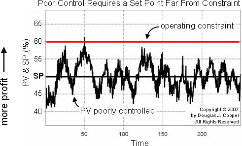
Controllers Reduce Variability
As shown in the plot below, a poorly controlled process can exhibit large variability in a measured process variable (e.g., temperature, pressure, level, flow, concentration) over time.
Suppose, as in this example, the measured process variable (PV) must not exceed a maximum value. And as is often the case, the closer we can run to this operating constraint, the greater our profit (note the vertical axis label on the plot).
To ensure our operating constraint limit is not exceeded, the operator-specified set point (SP), that is, the point where we want the control system to maintain our PV, must be set far from the constraint to ensure it is never violated. Note in the plot that SP is set at 50% when our PV is poorly controlled.
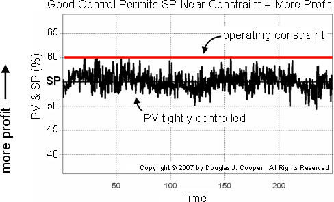
Below we see the same process with improved control.
There is significantly less variability in the measured PV, and as a result, the SP can be moved closer to the operating constraint.
With the SP in the plot below moved to 55%, the average PV is maintained closer to the specification limit
while still remaining below the maximum allowed value.
The result is increased profitability of our operation.
Terminology of Control
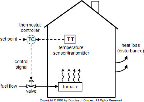
We establish the jargon for this site by discussing a home heating control system as illustrated below.
This is a simplistic example because a home furnace is either on or off. Most control challenges have a final control element (FCE), s
uch as a valve, pump or compressor, that can receive and respond to a complete range ofcontroller output (CO) signals
between full on and full off. This would include, for example, a valve that can be open 37% or a pump that can be running at 73%.
For our home heating process, the control objective is to keep the measured process variable (PV)
at the set point value (SP) in spite of unmeasured disturbances (D).
For our home heating system:
- PV = process variable is house temperature
- CO = controller output signal from thermostat to furnace valve
- SP = set point is the desired temperature set on the thermostat by the home owner
- D = heat loss disturbances from doors, walls and windows; changing outdoor temperature; sunrise and sunset; rain…
To achieve this control objective, the measured process variable is compared to the thermostat set point.
The difference between the two is the controller error, which is used in a control algorithm
such as a PID (proportional-integral-derivative) controller to compute a CO signal to the final control element (FCE).
The change in the controller output (CO) signal causes a response in the final control element (fuel flow valve),
which subsequently causes a change in the manipulated process variable (flow of fuel to the furnace).
If the manipulated process variable is moved in the right direction and by the right amount,
the measured process variable will be maintained at set point, thus satisfying the control objective.
This example, like all in process control, involves a measurement, computation and action:
- is the measured temp colder than set point (SP – PV > 0)? Then open the valve.
- is the measured temp hotter than set point (SP – PV < 0)? Then close the valve.
Note that computing the necessary controller action is based on controller error,
or the difference between the set point and the measured process variable, i.e.
e(t) = SP – PV (error = set point – measured process variable)
In a home heating process, control is an on/off or open/close decision.
And as outlined above, it is a straightforward decision to make.
The price of such simplicity, however, is that the capability to tightly regulate our measured PV is rather limited.
One situation not addressed above is the action to take when PV = SP (i.e., e(t) = 0).
And in industrial practice, we are concerned with variable position final control elements,
so the challenge elevates to computing:
- the direction to move the valve, pump, compressor, heating element…
- how far to move it at this moment
- how long to wait before moving it again
- whether there should be a delay between measurement and action
This site
This site offers information and discussion on proven methods and practices for PID (proportional-integral-derivative) control and related architectures such as cascade, feed forward, Smith predictors, multivariable decoupling, and similar traditional and advanced classical strategies.
Applications focus on processes with streams comprised of gases, liquids, powders, slurries and melts. As stated above, final control elements for these applications tend to be valves, variable speed pumps and compressors, and cooling and heating elements.
Industries that operate such processes include chemical, bio-pharma, oil and gas, paints and coatings, food and beverages, cement and coal, polymers and plastics, metals and materials, pulp and paper, personal care products, and more.
Components of a Control Loop
A controller seeks to maintain the measured process variable (PV) at set point (SP) in spite of unmeasured disturbances (D). The major components of a control system include a sensor, a controller and a final control element. To design and implement a controller, we must:
have identified a process variable we seek to regulate, be able to measure it (or something directly related to it) with a sensor, and be able to transmit that measurement as an electrical signal back to our controller, and have a final control element (FCE) that can receive the controller output (CO) signal, react in some fashion to impact the process (e.g., a valve moves), and as a result cause the process variable to respond in a consistent and predictable fashion.
Home Temperature Control
As shown below, the home heating control system described in this article
can be organized as a traditional control loop block diagram.
Block diagrams help us visualize the components of a loop and see how the pieces are connected.
A home heating system is simple on/off control with many of the components contained in a small box mounted on our wall.
Nevertheless, we introduce the idea of control loop diagrams by presenting a home heating system in the same way
we would a more sophisticated commercial control application.
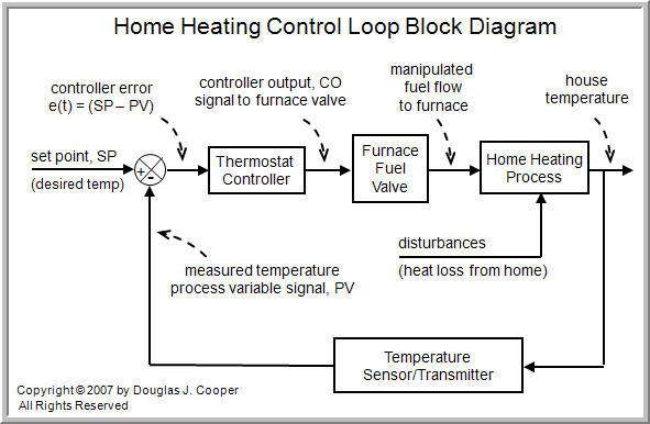
Starting from the far right in the diagram above, our process variable of interest is house temperature. A sensor, such as a thermistor in a modern digital thermostat, measures temperature and transmits a signal to the controller.
The measured temperature PV signal is subtracted from set point to compute controller error, e(t) = SP – PV. The action of the controller is based on this error, e(t).
In our home heating system, the controller output (CO) signal is limited to open/close for the fuel flowsolenoid valve (our FCE). So in this example, if e(t) = SP – PV > 0, the controller signals to open the valve. If e(t) = SP – PV < 0, it signals to close the valve. As an aside, note that there also must be a safety interlock to ensure that the furnace burner switches on and off as the fuel flow valve opens and closes.
As the energy output of the furnace rises or falls, the temperature of our house increases or decreases and a feedback loop is complete. The important elements of a home heating control system can be organized like any commercial application:
- Control Objective: maintain house temperature at SP in spite of disturbances
- Process Variable: house temperature
- Measurement Sensor: thermistor; or bimetallic strip coil on analog models
- Measured Process Variable (PV) Signal: signal transmitted from the thermistor
- Set Point (SP): desired house temperature
- Controller Output (CO): signal to fuel valve actuator and furnace burner
- Final Control Element (FCE): solenoid valve for fuel flow to furnace
- Manipulated Variable: fuel flow rate to furnace
- Disturbances (D): heat loss from doors, walls and windows; changing outdoor temperature; sunrise and sunset; rain…
A General Control Loop and Intermediate Value Control
The home heating control loop above can be generalized into a block diagram pertinent to all feedback control loops as shown below

Both diagrams above show a closed loop system based on negative feedback. That is, the controller takes actions that counteract or oppose any drift in the measured PV signal from set point.
While the home heating system is on/off, our focus going forward shifts to intermediate value control loops. An intermediate value controller can generate a full range of CO signals anywhere between full on/off or open/closed. The PI algorithm and PID algorithm are examples of popular intermediate value controllers.
To implement intermediate value control, we require a sensor that can measure a full range of our process variable, and a final control element that can receive and assume a full range of intermediate positions between full on/off or open/closed. This might include, for example, a process valve, variable speed pump or compressor, or heating or cooling element.
Note from the loop diagram that the process variable becomes our official PV only after it has been measured by a sensor and transmitted as an electrical signal to the controller. In industrial applications. these are most often implemented as 4-20 milliamps signals, though commercial instruments are available that have been calibrated in a host of amperage and voltage units.
With the loop closed as shown in the diagrams, we are said to be in automatic mode and the controller is making all adjustments to the FCE. If we were to open the loop and switch to manual mode, then we would be able to issue CO commands through buttons or a keyboard directly to the FCE. Hence:
• open loop = manual mode
• closed loop = automatic mode
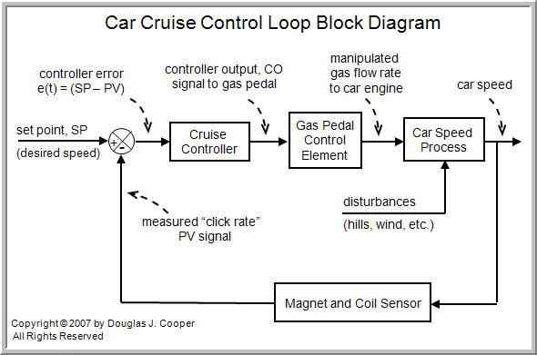
Cruise Control and Measuring Our PV
Cruise control in a car is a reasonably common intermediate value control system. For those who are unfamiliar with cruise control, here is how it works.
We first enable the control system with a button on the car instrument panel. Once on the open road and at our desired cruising speed, we press a second button that switches the controller from manual mode (where car speed is adjusted by our foot) to automatic mode (where car speed is adjusted by the controller).
The speed of the car at the moment we close the loop and switch from manual to automatic becomes the set point. The controller then continually computes and transmits corrective actions to the gas pedal (throttle) to maintain measured speed at set point.
It is often cheaper and easier to measure and control a variable directly related to the process variable of interest. This idea is central to control system design and maintenance. And this is why the loop diagrams above distinguish between our “process variable” and our “measured PV signal.”
Cruise control serves to illustrate this idea. Actual car speed is challenging to measure. But transmission rotational speed can be measured reliably and inexpensively. The transmission connects the engine to the wheels, so as it spins faster or slower, the car speed directly increases or decreases.
Thus, we attach a small magnet to the rotating output shaft of the car transmission and a magnetic field detector (loops of wire and a simple circuit) to the body of the car above the magnet. With each rotation, the magnet passes by the detector and the event is registered by the circuitry as a “click.” As the drive shaft spins faster or slower, the click rate and car speed increase or decrease proportionally.
So a cruise control system really adjusts fuel flow rate to maintain click rate at the set point value. With this knowledge, we can organize cruise control into the essential design elements:
- Control Objective: maintain car speed at SP in spite of disturbances
- Process Variable: car speed
- Measurement Sensor: magnet and coil to clock drive shaft rotation
- Measured Process Variable (PV) Signal: “click rate” signal from the magnet and coil
- Set Point (SP): desired car speed, recast in the controller as a desired click rate
- Controller Output (CO): signal to actuator that adjusts gas pedal (throttle)
- Final Control Element (FCE): gas pedal position
- Manipulated Variable: fuel flow rate
- Disturbances (D): hills, wind, curves, passing trucks…
The traditional block diagram for cruise control is thus:
Instruments Should be Fast, Cheap and Easy
The above magnet and coil “click rate = car speed” example introduces the idea that when purchasing an instrument for process control, there are wider considerations that can make a loop faster, easier and cheaper to implement and maintain. Here is a “best practice” checklist to use when considering an instrument purchase:
- Low cost
- Easy to install and wire
- Compatible with existing instrument interface
- Low maintenance
- Rugged and robust
- Reliable and long lasting
- Sufficiently accurate and precise
- Fast to respond (small time constant and dead time)
- Consistent with similar instrumentation already in the plant
Process Data, Dynamic Modeling and a Recipe for Profitable Control
It is best practice to follow a formal procedure or “recipe” when designing and tuning a PID (proportional-integral-derivative) controller. A recipe-based approach is the fastest method for moving a controller into operation. And perhaps most important, the performance of the controller will be superior to a controller tuned using a guess-and-test or trial-and-error method.
Additionally, a recipe-based approach overcomes many of the concerns that make control projects challenging in a commercial operating environment. Specifically, the recipe-based method causes less disruption to the production schedule, wastes less raw material and utilities, requires less personnel time, and generates less off-spec product.
The recipe for success is short:
- Establish the design level of operation (DLO), defined as the expected values for set point and major disturbances during normal operation
- Bump the process and collect controller output (CO) to process variable (PV) dynamic process data around this design level
- Approximate the process data behavior with a first order plus dead time (FOPDT) dynamic model
- Use the model parameters from step 3 in rules and correlations to complete the controller design and tuning.
We explore each step of this recipe in detail in other articles on this site. For now, we introduce some initial thoughts about steps 2 and 4.
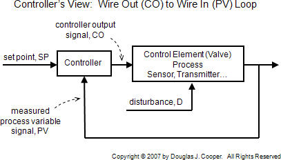
Step 2: Bumping Our Process and Collecting CO to PV Data
From a controller’s view, a complete control loop goes from wire out to wire in as shown below.
Whenever we mention controller output (CO) or process variable (PV) data anywhere on this site,
we are specifically referring to the data signals exiting and entering our controller at the wire termination interface.
To generate CO to PV data, we bump our process. That is, we step or pulse the CO (or the set point if in automatic mode as discussed here) and record PV data as the process responds. Here are three basic rules we follow in all of our examples:
• Start with the process at steady state and record everything
The point of bumping the CO is to learn about the cause and effect relationship between it and the PV. With the plant initially at steady state, we are starting with a clean slate. The dynamic behavior of the process is then clearly isolated as the PV responds. It is important that we start capturing data before we make the initial CO bump and then sample and record quickly as the PV responds.
• Make sure the PV response dominates the process noise
When performing a bump test, it is important that the CO moves far enough and fast enough to force a response that clearly dominates any noise or random error in the measured PV signal. If the CO to PV cause and effect response is clear enough to see by eye on a data plot, we can be confident that modern softwarecan model it.
• The disturbances should be quiet during the bump test
We desire that the dynamic test data contain PV response data that has been clearly, and in the ideal world exclusively, forced by changes in the CO.
Data that has been corrupted by unmeasured disturbances is of little value for controller design and tuning. The model (see below) will then incorrectly describe the CO to PV cause and effect relationship. And as a result, the controller will not perform correctly. If we are concerned that a disturbance event has corrupted test data, it is conservative to rerun the test.
Step 4: Using Model Parameters For Design and Tuning
The final step of the recipe states that once we have obtained model parameters that approximate the dynamic behavior of our process, we can complete the design and tuning of our PID controller.
We look ahead at this last step because this is where the payoff of the recipe-based approach is clear. To establish the merit, we assume for now that we have determined the design level of operation for our process (step 1), we have collected a proper data set rich in dynamic process information around this design level (step 2), and we have approximated the behavior revealed in the process data with a first order plus dead time (FOPDT) dynamic model (step 3).
Thankfully, we do not need to know what a FOPDT model is or even what it looks like. But we do need to know about the three model parameters that result when we fit this approximating model to process data.
The FOPDT (first order plus dead time) model parameters, listed below, tell us important information about the measured process variable (PV) behavior whenever there is a change in the controller output (CO) signal:
- process gain, Kp (tells the direction and how far PV will travel)
- process time constant, Tp (tells how fast PV moves after it begins its response)
- process dead time, Өp (tells how much delay before PV first begins to respond)
Aside: we do not need to understand differential equations to appreciate the articles on this site. But for those interested, we note that the first order plus dead time (FOPDT) dynamic model has the form:
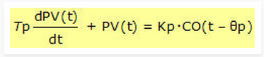
Where:
PV(t) = measured process variable as a function of time
CO(t – Өp) = controller output signal as a function of time and shifted by Өp
Өp = process dead time
t = timeThe other variables are as listed above this box. It is a first order differential equation because it has one derivative with one time constant, Tp. It is called a first order plus dead time equation because it also directly accounts for a delay or dead time, Өp, in the CO(t) to PV(t) behavior.
We study what these three model parameters are and how to compute them in other articles, but here is why process gain, Kp, process time constant, Tp, and process dead time, Өp, are all important:
• Tuning
These three model parameters can be plugged into proven correlations to directly compute P-Only, PI, PID, and PID with CO Filter tuning values. No more trial and error. No more tweaking our way to acceptable control. Great performance can be readily achieved with the step by step recipe listed above.
• Controller Action
Before implementing our controller, we must input the proper direction our controller should move to correct for growing errors. Some vendors use the term “reverse acting” and “direct acting.” Others use terms like “up-up” and “up-down” (as CO goes up, then PV goes up or down). This specification is determined solely by the sign of the process gain, Kp.
• Loop Sample Time, T
Process time constant, Tp, is the clock of a process. The size of Tp indicates the maximum desirable loop sample time. Best practice is to set loop sample time, T, at 10 times per time constant or faster (T ≤ 0.1Tp). Sampling faster will not necessarily provide better performance, but it is a safer direction to move if we have any doubts. Sampling too slowly will have a negative impact on controller performance. Sampling slower than five times per time constant will lead to degraded performance.
• Dead Time Problems
As dead time grows larger than the process time constant (Өp > Tp), the control loop can benefit greatly from a model based dead time compensator such as a Smith predictor. The only way we know if Өp > Tp is if we have followed the recipe and computed the parameters of a FOPDT model.
• Model Based Control
If we choose to employ a Smith predictor, a dynamic feed forward element, a multivariable decoupler, or any other model based controller, we need a dynamic model of the process to enter into the control computer. The FOPDT model from step 2 of the recipe is often appropriate for this task.
Fundamental to Success
With tuning values, loop specifications, performance diagnostics and advanced control all dependent on knowledge of a dynamic model, we begin to see that process gain, Kp; process time constant, Tp; and process dead time, Өp; are parameters of fundamental importance to success in process control.
Sample Time Impacts Controller Performance
There are two sample times, T, used in process controller design and tuning.
One is the control loop sample time that specifies how often the controller samples the measured process variable (PV) and then computes and transmits a new controller output (CO) signal.
The other is the rate at which CO and PV data are sampled and recorded during a bump test of our process. Bump test data is used to design and tune our controller prior to implementation.
In both cases, sampling too slow will have a negative impact on controller performance. Sampling faster will not necessarily provide better performance, but it is a safer direction to move if we have any doubts.
Fast and slow are relative terms defined by the process time constant, Tp. Best practice for both control loop sample time and bump test data collection are the same:
Best Practice: Sample time should be 10 times per process time constant or faster (T ≤ 0.1Tp).
We explore this “best practice” rule in a detailed study here. This study employs some fairly advanced concepts, so it is placed further down in the Table of Contents.
Yet perhaps we can gain an appreciation for how sample time impacts controller design and tuning with this thought experiment:
Suppose you see me standing on your left. You close your eyes for a time, open them, and now I am standing on your right. Do you know how long I have been at my new spot? Did I just arrive or have I been there for a while? What path did I take to get there? Did I move around in front or in back of you? Maybe I even jumped over you?

Now suppose your challenge is to keep your hands at your side until I pass by, and just as I do, you are to reach out and touch me. What are your chances with your eyes closed (and loud music is playing so you cannot hear me)?

Now lets say you are permitted to blink open your eyes briefly once per minute. Do you think you will have a better chance of touching me? How about blinking once every ten seconds? Clearly, as you start blinking say, two or three times a second, the task of touching me becomes easy. That’s because you are sampling fast enough to see my “process” behavior fully and completely.
Based on this thought experiment, sampling too slow is problematic and sampling faster is generally better.
Keep in mind the “T ≤ 0.1Tp” rule as we study PID control. This applies both to sampling during data collection, and the “measure and act” loop sample time when we implement our controller.
Step Test Data From the Heat Exchanger Process
A previous article presented the first order plus dead time (FOPDT) dynamic model and discussed how this model, when used to approximate the controller output (CO) to process variable (PV) behavior of proper data from our process, yields the all-important model parameters:
- process gain, Kp (tells the direction and how far PV will travel)
- process time constant, Tp (tells how fast PV moves after it begins its response)
- process dead time, Өp (tells how much delay before PV first begins to respond)
The previous articles also mentioned that these FOPDT model parameters can be used to determine PID tuning values, proper sample time, whether the controller should be direct or reverse acting, whether dead time is large enough to cause concern, and more.
A Hands-On Study
There is an old saying (a Google search shows a host of attributed authors) that goes something like this: I hear and I forget, I see and I remember, I do and I understand.
Since our goal is to understand, this means we must “do.” To that end, we take a hands-on approach in this case study that will help us appreciate what each FOPDT model parameter is telling us about our process and empower us to act accordingly as we explore best practices for controller design and tuning.
To proceed, we require a process we can manipulate freely. We start with a heat exchanger because they are common to a great many industries.
Heat Exchanger Process
The heat exchanger we will study is really a process simulation from commercial software. The simulation is developed from first-principles theory, so its response behavior is realistic. The benefit of a simulation is that we can manipulate process variables whenever and however we desire without risk to people or profit.
The heat exchanger is shown below (click for a large view) in manual mode (also called open loop). Its behavior is that of a counter-current, shell and tube, hot liquid cooler.
The measured process variable is the hot liquid temperature exiting the exchanger on the tube side. To regulate this hot exit temperature, the controller moves a valve to manipulate the flow rate of a cooling liquid entering on the shell side.
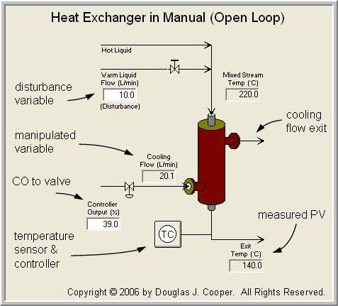
The hot tube side and cool shell side liquids do not mix. Rather, the cooling liquid surrounds the hot tubes and pulls off heat energy as it passes through the exchanger. As the flow rate of cooling liquid around the tubes increases (as the valve opens), more heat is removed and the temperature of the exiting hot liquid decreases.
A side stream of warm liquid combines with the hot liquid entering the exchanger and acts as a disturbance to our process in this case study. As the warm stream flow rate increases, the mixed stream temperature decreases (and vice versa).
Shown below is the heat exchanger in automatic mode (also called closed loop) using the standard nomenclature for this site.
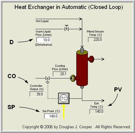
The measured process variable (PV) is the hot liquid temperature exiting the exchanger. The controller output (CO) signal moves a valve to manipulate the flow rate of cooling liquid on the shell side to maintain the PV at set point (SP). The warm liquid flow acts as a disturbance (D) to the process.
Generating Step Test Data
To fit a FOPDT (first order plus dead time) model to dynamic process data using hand calculations, we will be reading numbers off of a plot. Such a graphical analysis technique can only be performed on step test data collected in manual mode (open loop).
Practitioner’s Note: operations personnel can find switching to manual mode and performing step tests to be unacceptably disruptive, especially when the production schedule is tight. It is sometimes easier to convince them to perform a closed loop (automatic mode) pulse test, but such data must be analyzed by software and this reduces our “doing” to simply “seeing” software provide answers.
To generate our dynamic process step test data, wait until the CO and PV appear to be as steady as is reasonable for the process under study. Then, after confirming we are in manual mode, step the CO to a new value.
The CO step must be large enough and sudden enough to cause the PV to move in a clear response that dominates all noise in the measurement signal. Data collection must begin before the CO step is implemented and continue until the PV reaches a new steady state.
The plot below shows dynamic step test data from the heat exchanger. Note that the PV signal (the upper trace in the plot) includes a small amount of random measurement noise. This is added in the simulation to create a more realistic process behavior.
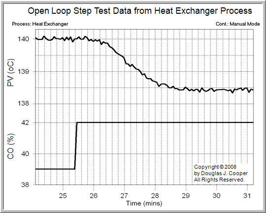
As shown in the plot, the CO is initially constant at 39% while the exit temperature PV is steady at about 140 °C. The CO is then stepped from 39% up to 42%.
The step increase in CO causes the valve to open, increasing the flow rate of cooling liquid into the shell side of the exchanger. The additional cooling liquid causes the measured PV (exit temperature on the tube side) to decrease from its initial steady state value of 140 °C down to a new value of about 138.4 °C.
We will refer back to the this dynamic process test data in future articles as we work through the details of computing process gain, Kp; process time constant, Tp; and process dead time, Өp.
Practitioner’s Note: the heat exchanger graphic shows that this process has one disturbance variable, D. It is a side stream of warm liquid that mixes with the hot liquid on the tube side. When generating the step test data above, disturbance D is held constant.Yet real processes can have many disturbances, and by their very nature, disturbances are often beyond our ability to monitor, let alone control. While quiet disturbances are something we can guarantee in a simulation, we may not be so lucky in the plant. Yet to accurately model the dynamics of a process, it is essential that the influential disturbances remain quiet when generating dynamic process test data.Whether the disturbances have remained quiet during a dynamic test is something you must “know” about your process. Otherwise, you should not be adjusting any controller settings.
To appreciate this sentiment, recognize that you “know” when your car is acting up. You can sense when it shows a slight but clearly different behavior that needs attention. Someone planning to adjust the controllers in an industrial operation should have this same level of familiarity with their process.
Process Gain Is The “How Far” Variable
Step 3 of our controller design and tuning recipe is to approximate the often complex behavior contained in our dynamic process test data with a simple first order plus dead time (FOPDT) dynamic model.
In this article we focus on process gain, Kp, and seek to understand what it is, how it is computed, and what it implies for controller design and tuning. Corresponding articles present details of the other two FOPDT model parameters: process time constant, Tp; and process dead time, Өp.
Heat Exchanger Step Test Data
We explore Kp by analyzing step test data from a heat exchanger. The heat exchanger is a realistic simulation where the measured process variable (PV) is the temperature of hot liquid exiting the exchanger. To regulate this PV, the controller output (CO) signal moves a valve to manipulate the flow rate of a cooling liquid into the exchanger.
The step test data below was generated by moving the process from one steady state to another. As shown, the CO was stepped from 39% up to 42%, causing the measured PV to decrease from 140 °C down to approximately 138.4 °C.

Computing Process Gain
Kp describes the direction PV moves and how far it travels in response to a change in CO. It is based on the difference in steady state values. The path or length of time the PV takes to get to its new steady state does not enter into the Kp calculation.
Thus, Kp is computed:

where ΔPV and ΔCO represent the total change from initial to final steady state.
Aside: the assumptions implicit in the discussion above include that:
- the process is properly instrumented as a CO to PV pair,
- major disturbances remained reasonably quiet during the test, and
- the process itself is self regulating. That is, it naturally seeks to run at a steady state if left uncontrolled and disturbances remain quiet.
Most, but certainly not all, processes are self regulating.
Certain configurations of something as simple as liquid level in a pumped tank can be non-self regulating.
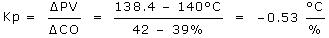
Reading numbers off the above plot:
The CO was stepped from 39% up to 42%, so the ΔCO = 3%.
The PV was initially steady at 140 °C and moved down to a new steady state value of 138.4 °C. Since it decreased, the ΔPV = –1.6 °C.
Using these ΔCO and ΔPV values in the Kp equation above, the process gain for the heat exchanger is computed:
Practitioner’s Note: Real plant data is rarely as clean as that shown in the plot above and we should be cautious not to try and extract more information from our data than it actually contains. When used in tuning correlations, rounding the Kp value to –0.5 °C/% will provide virtually the same performance.
Kp Impacts Control
Process gain, Kp, is the “how far” variable because it describes how far the PV will travel for a given change in CO. It is sometimes called the sensitivity of the process.
If a process has a large Kp, then a small change in the CO will cause the PV to move a large amount. If a process has a small Kp, the same CO change will move the PV a small amount.
As a thought experiment, let’s suppose a disturbance moves our measured PV away from set point (SP). If the process has a large Kp, then the PV is very sensitive to CO changes and the controller should make small CO moves to correct the error. Conversely, if the process has a small Kp, then the controller needs to make large CO actions to correct the same error.
This is the same as saying that a process with a large process gain, Kp, should have a controller with a small controller gain, Kc (and vice versa).
Looking ahead to the PI tuning correlations we will use in our case studies:

Where:
Kc = controller gain, a tuning parameter
Ti = reset time, a tuning parameter
Notice that in the Kc correlation, a large Kp in the denominator will yield a small Kc value (that is, Kc is inversely proportional to Kp). Thus, the tuning correlation tells us the same thing as our thought experiment above.
Sign of Kp Tells Direction
The sign of Kp tells us the direction the PV moves relative to the CO change. The negative value found above means that as the CO goes up, the PV goes down. We see this “up-down” relationship in the plot. For a process where a CO increase causes the PV to move up, the Kp would be positive and this would be an “up-up” process.
When implementing a controller, we need to know if our process is up-up or up-down. If we tell the controller the wrong relationship between CO actions and the direction of the PV responses, our mistake may prove costly. Rather than correcting for errors, the controller will quickly amplify them as it drives the CO signal, and thus the valve, pump or other final control element (FCE), to the maximum or minimum value.
Units of Kp
If we are computing Kp and want the results to be meaningful for control, then we must be analyzing wire out to wire in CO to PV data as used by the controller.
The heat exchanger data plot indicates that the data arriving on the PV wire into the controller has been scaled (or is being scaled in the controller) into units of temperature. And this means the the controller gain, Kc, needs to reflect the units of temperature as well.
This may be confusing, at least initially, since most commercial controllers do not require that units be entered. The good news is that, as long as our computations use the same “wire out to wire in” data as collected and displayed by our controller, the units will be consistent and we need not dwell on this issue.
Aside:
for the Kc tuning correlation above, the units of time (dead time and time constants) cancel out. Hence, the controller gain, Kc, will have the reciprocal or inverse units of Kp. For the heat exchanger, this means Kc has units of %/°C.With modern computer control systems, scaling for unit conversions is becoming more common in the controller signal path. Sometimes a display has been scaled but the signal in the loop path has not. You must pay attention to this detail and make sure you are using the correct units in your computations. There is more discussion in this article.It has been suggested that the gain of some controllers do not have units since both the CO and PV are in units of %. Actually, the Kc will have units of “% of CO signal” divided by “% of PV signal,” which mathematically do not cancel out.
Practitioner’s Note:
Step test data is practical in the sense that all model fitting computations can be performed by reading numbers off of a plot. However, when dealing with production processes, operations personnel tend to prefer quick “bumps” rather than complete step tests.Step tests move the plant from one steady state to another. This takes a long time, may have safety implications, and can create expensive off-spec product. Pulse and doublet tests are examples of quick bumps that returns our plant to desired operating conditions as soon as the process data shows a clear response to a controller output (CO) signal change.Getting our plant back to a safe, profitable operation as quickly as possible is a popular concept at all levels of operation and management. Using pulse tests requires the use of inexpensive commercial software to analyze the bump test results, however.
Process Time Constant is The “How Fast” Variable
Step 3 of our controller design and tuning recipe is to approximate the often complex behavior contained in our dynamic process test data with a simple first order plus dead time (FOPDT) dynamic model.
In this article we focus on process time constant, Tp, and seek to understand what it is, how it is computed, and what it implies for controller design and tuning. Corresponding articles present details of the other two FOPDT model parameters: process gain, Kp; and process dead time, Өp.
Heat Exchanger Step Test Data
We seek to understand Tp by analyzing step test data from a heat exchanger. The heat exchanger is a realistic simulation where the measured process variable (PV) is the temperature of hot liquid exiting the exchanger. To regulate this PV, the controller output (CO) moves a valve to manipulate the flow rate of a cooling liquid into the exchanger.
The step test data below was generated by moving the process from one steady state to another. As shown, the CO was stepped from 39% up to 42%, causing the measured PV to decrease from 140 °C down to approximately 138.4 °C.
Time Constant in Words
In general terms, the time constant, Tp, describes how fast the PV moves in response to a change in the CO.
The time constant must be positive and it must have units of time. For controllers used on processes comprised of gases, liquids, powders, slurries and melts, Tp most often has units of minutes or seconds.
We can be more precise in our word definition if we restrict ourselves to step test data such as that shown in the plot above. Please recognize that while it is easier to describeTp in words using step test data, it is a parameter that always describes “how fast” PV moves in response to any sort of CO change.
Step test data implies that the process is in manual mode (open loop) and initially at steady state. A step in the CO has forced a response in the PV, which moves from its original steady state value to a final steady state.
With these restrictions, we compute Tp in five steps:
1. Determine ΔPV, the total change that is going to occur in PV, computed as “final minus initial steady state”
2. Compute the value of the PV that is 63% of the total change that is going to occur, or “initial steady state PV + 0.63(ΔPV)”
3. Note the time when the PV passes through the 63% point of “initial steady state PV + 0.63(ΔPV)”
4. Subtract from it the time when the “PV starts a clear response” to the step change in the CO
5. The passage of time from step 4 minus step 3 is the process time constant, Tp.
Summarizing in one sentence, for step test data, Tp is the time that passes from when the PV shows its first response to the CO step, until when the PV reaches 63% of the total DPV change that is going to occur.
Computing Tp for the Heat Exchanger
Following the steps above for the heat exchanger step test data:
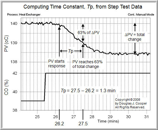
1. The PV was initially steady at 140 °C and moved down to a final steady state of 138.4 °C. The total change,ΔPV, is “final minus initial steady state” or:
ΔPV = 138.4 – 140 = –1.6 °C
2. The value of the PV that is 63% of this total change is “initial steady state PV + 0.63ΔPV” or:
initial PV + 0.63(ΔPV) = 140 + 0.63(–1.6)
= 140 – 1.0
= 139 °C
3. From the plot, the time when the PV passes through the “initial steady state PV + 0.63ΔPV” point of 139 °C is:
Time to 0.63(ΔPV) = Time to 139 °C
= 27.5 min
4. From the plot (see the following Practitioner’s Note), the time when the “PV starts a response” to the CO step is:
Time PV response starts = 26.2 min
5. The time constant is “time to 63%(ΔPV)” minus “time PV response starts” or:
Tp = 27.5 – 26.2 = 1.3 min
A detailed derivation of the 63% rule is provided in this pdf.
Dead Time Is The “How Much Delay” Variable
Step 3 of our controller design and tuning recipe is to approximate the often complex behavior contained in our dynamic process test data with a simple first order plus dead time (FOPDT) dynamic model.
In this article we focus on process dead time, Өp, and seek to understand what it is, how it is computed, and what it implies for controller design and tuning. Corresponding articles present details of the other two FOPDT model parameters: process gain, Kp; and process time constant, Tp.
Dead Time is the Killer of Control
Dead time is the delay from when a controller output (CO) signal is issued until when the measured process variable (PV) first begins to respond. The presence of dead time,Өp, is never a good thing in a control loop.
Think about driving your car with a dead time between the steering wheel and the tires. Every time you turn the steering wheel, the tires do not respond for, say, two seconds. Yikes.
For any process, as Өp becomes larger, the control challenge becomes greater and tight performance becomes more difficult to achieve. “Large” is a relative term and this is discussed later in this article.
Causes for Dead Time
Dead time can arise in a control loop for a number of reasons:
- Control loops typically have “sample and hold” measurement instrumentation that introduces a minimum dead time of one sample time, T, into every loop. This is rarely an issue for tuning, but indicates that every loop has at least some dead time.
- The time it takes for material to travel from one point to another can add dead time to a loop. If a property (e.g. a concentration or temperature) is changed at one end of a pipe and the sensor is located at the other end, the change will not be detected until the material has moved down the length of the pipe. The travel time is dead time. This is not a problem that occurs only in big plants with long pipes. A bench top process can have fluid creeping along a tube. The distance may only be an arm’s length, but a low enough flow velocity can translate into a meaningful delay.
- Sensors and analyzer can take precious time to yield their measurement results. For example, suppose a thermocouple is heavily shielded so it can survive in a harsh environment. The mass of the shield can add troublesome delay to the detection of temperature changes in the fluid being measured.
- Higher order processes have an inflection point that can be reasonably approximated as dead time for the purpose of controller design and tuning. Note that modeling for tuning with the simple FOPDT form is different from modeling for simulation, where process complexities should be addressed with more sophisticated model forms (all subjects for future articles).
Sometimes dead time issues can be addressed through a simple design change. It might be possible to locate a sensor closer to the action, or perhaps switch to a faster responding device. Other times, the dead time is a permanent feature of the control loop and can only be addressed through detuning or implementation of a dead time compensator (e.g. Smith predictor).
Heat Exchanger Test Data
We seek to understand Kp by analyzing step test data from a heat exchanger. The heat exchanger is a realistic simulation where the measured process variable (PV) is the temperature of hot liquid exiting the exchanger. To regulate this PV, the controller output (CO) moves a valve to manipulate the flow rate of a cooling liquid into the exchanger.
The step test data below (click for a larger view) was generated by moving the process from one steady state to another. In particular, CO was stepped from 39% up to 42%, causing the measured PV to decrease from 140 °C down to approximately 138.4 °C.
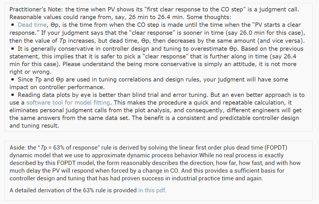
Computing Dead Time
Estimating dead time, Өp, from step test data is a three step procedure:
1. Locate the point in time when the “PV starts a clear response” to the step change in the CO. This is the same point we identified when we computed Tp in the previous article.
2. Locate the point in time when the CO was stepped from its original value to its new value.
3. Dead time, Өp, is the difference in time of step 1 minus step 2.
Applying the three step procedure to the step test plot above:
1. As we had determined in the previous Tp article, the PV starts a clear response to the CO step at 26.2 min.
2. Reading off the plot, the CO step occurred at 25.4 min, and thus,
3. Өp = 26.2 – 25.4 = 0.8 min
We analyze step test data here to make the computation straightforward, but please recognize that dead time describes “how much delay” occurs from when any sort of CO change is made until when the PV first responds to that change.
Like a time constant, dead time has units of time and must always be positive. For the types of processes explored on this site (streams comprised of gasses, liquids, powders, slurries and melts), dead time is most often expressed in minutes or seconds.
During a dynamic analysis study, it is best practice to express Tp and Өp in the same units (e.g. both in minutes or both in seconds). The tuning correlations and design rules assume consistent units. Control is challenging enough without adding computational error to our problems.
Implications for Control
• Dead time, Өp, is large or small only in comparison to Tp, the clock of the process. Tight control becomes more challenging when Өp > Tp. As dead time becomes much greater than Tp, a dead time compensator such as a Smith predictor offers benefit. A Smith predictor employs a dynamic process model (such as an FOPDT model) directly within the architecture of the controller. It requires additional engineering time to design, implement and maintain, so be sure the loop is important to safety or profitability before undertaking such a project.
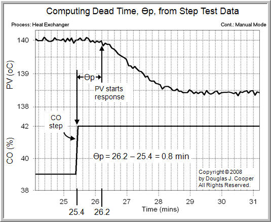
• It is more conservative to overestimate dead time when the goal is tuning. ComputingӨp requires a judgment of when the “PV starts a clear response.” If your judgment says that the “clear response” is sooner in time (maybe you choose 26.0 min for this case), then Tp increases, but dead time, Өp, decreases by the same amount (and vice versa). We can see the impact this has by looking ahead to the PI tuning correlations:
Where:
Kc = controller gain, a tuning parameter
Ti = reset time, a tuning parameter
Since Өp is in the denominator of the Kc correlation, as dead time gets larger, the controller gain gets smaller. A smaller Kc implies a less active controller. Overly aggressive controllers cause more trouble than sluggish controllers, at least in the first moments after being put into automatic. Hence, a larger dead time estimate is a more cautious or conservative estimate.
Practitioner’s Note on the “Өp,min = T” Rule for Controller Tuning:Consider that all controllers measure, act, then wait until next sample time; measure, act, then wait until next sample time. This “measure, act, wait” procedure has a delay (or dead time) of one sample time, T, built naturally into its structure.
Thus, the minimum dead time, Өp, in any real control implementation is the loop sample time, T. Dead time can certainly be larger than T (and it usually is), but it cannot be smaller.Thus, if our model fit yields Өp < T (a dead time that is less than the controller sample time), we must recognize that this is an impossible outcome. Best practice in such a situation is to substitute Өp = T everywhere when using our controller tuning correlations and other design rules.
This is the “Өp,min = T” rule for controller tuning. Read more details about the impact of sample time on controller design and tuning in this article.
The Gravity Drained Tanks Process
Self Regulating vs Integrating Process Behavior
This case study considers the control of liquid level in a gravity drained tanks process. Like the heat exchanger, the gravity drained tanks displays a typical self regulating process behavior. That is, the measured process variable (PV) naturally seeks a steady operating level if the controller output (CO) and major disturbances are held constant for a sufficient length of time.
It is important to recognize that not all processes, and especially not all liquid level processes, exhibit a self regulating behavior. Liquid level control of a pumped tankprocess, for example, displays a classical integrating (or on-self-regulating) behavior.
The control of integrating processes presents unique challenges that we will explore in later articles. For now, it is enough to recognize that controller design and tuning for integrating processes has special considerations.
We note that, like the heat exchanger and pumped tank process, the gravity drained tanks case study is a sophisticated simulation derived from first-principles theory and available in commercial software. Simulations let us study different ideas without risking safety or profit. Yet the rules and procedures we develop here are directly applicable to the broad world of real processes with streams comprised of liquids, gases, powders, slurries and melts.
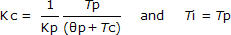
Gravity Drained Tanks Process
The gravity drained tanks process, shown below in manual mode (click for a large view), is comprised of two tanks stacked one above the other. They are essentially two drums or barrels with holes punched in the bottom.
A variable position control valve manipulates the inlet flow rate feeding the upper tank. The liquid drains freely out through the hole in the bottom of the upper tank to feed the lower tank. From there, the liquid exits either by an outlet drain (another free-draining hole) or by a pumped flow stream.
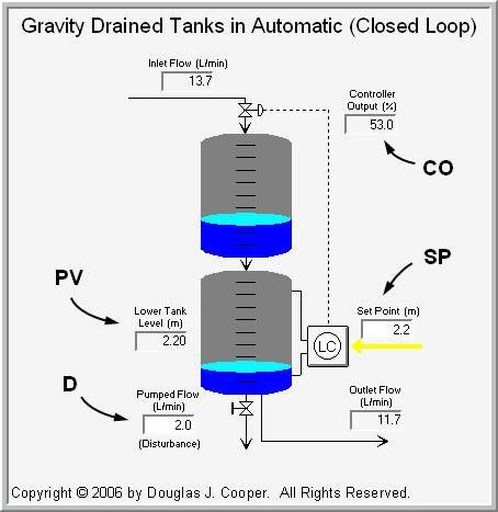
The next graphic (click for a large view) shows the process in automatic mode using our standard nomenclature.
The measured process variable (PV) is liquid level in the lower tank. The controller output (CO) adjusts the valve to maintain the PV at set point (SP).
Aside: The graphic shows tap lines out of the top and bottom of the lower tank and entering the level sensor/controller. This configuration hints at the use of pressure drop as the level measurement method. As we discuss here, we often choose to use sensors that are inexpensive to purchase, install and maintain to monitor parameters related to the actual variable of interest. While our trend plots in this case study show liquid level, our true measured variable is pressure drop across the liquid inventory in the tank. A simple multiplier block translates the weight of liquid pushing on the bottom tap into this level measurement display.
So, for example, if the liquid level in the lower tank is below set point:
- the controller opens the valve some amount,
- increasing the flow rate into the upper tank,
- raising the liquid level in the upper tank,
- increasing the pressure near the drain hole,
- raising the liquid drain rate into the lower tank,
- thus increasing the liquid level in the lower tank.
The Disturbance Stream
As shown in the above graphic, the pumped flow stream out of the lower tank acts as a disturbance to this process. The disturbance flow (D) is controlled independently, as if by another process (which is why it is a disturbance to our process).
Because the pumped flow rate, D, runs through a positive displacement pump, it is not affected by liquid level, though it drops to zero if the tank empties.
When D increases (or decreases), the measured PV level quickly falls (or rises) in response.
Process Behavior is Nonlinear
The dynamic behavior of this process is reasonably intuitive. Increase the inlet flow rate into the upper tank and the liquid level in the lower tank eventually rises to a new value. Decrease the inlet flow rate and the liquid level falls.
Gravity driven flows are proportional to the square root of the hydrostatic head, or height of liquid in a tank. As a result, the dynamic behavior of the process is modestly nonlinear. This is evident in the open loop response plot below (click for a larger view).

As shown above, the CO is stepped in equal increments, yet the response shape of the PV clearly changes as the level in the tank rises. The consequence of this nonlinear behavior is that a controller designed to give desirable performance at one operating level may not give desirable performance at another level.
Modeling Dynamic Process Behavior
We next explore dynamic modeling of process behavior for the gravity drained tanks.
Dynamic “Bump” Testing Of The Gravity Drained Tanks Process
We introduced the gravity drained tanks process in a previous article and established that it displays a self regulating behavior. We also learned that it exhibits a nonlinear behavior, though to a lesser degree than that of the heat exchanger.
Our control objective is to maintain liquid level in the lower tank at set point in spite of unplanned and unmeasured disturbances. The controller will achieve this by manipulating the inlet flow rate into the upper tank.
To proceed, we follow our controller design and tuning recipe:
- Establish the design level of operation (DLO), defined as the expected values for set point and major disturbances during normal operation
- Bump the process and collect controller output (CO) to process variable (PV) dynamic process data around this design level
- Approximate the process data behavior with a first order plus dead time (FOPDT) dynamic model to obtain estimates for process gain, Kp (how far variable), process time constant, Tp (how fast variable), and the process dead time, {U+04E8}p (with how much delay variable).
- Use the model parameters from step 3 in rules and correlations to complete the controller design and tuning.
Step 1: Design Level of Operation (DLO)
Nonlinear behavior is a common characteristic of processes with streams comprised of liquids, gases, powders, slurries and melts. Nonlinear behavior implies that Kp, Tp and/or Өp changes as operating level changes.
Since we use Kp, Tp and Өp values in correlations to complete the controller design and tuning, the fact that they change gives us pause. It implies that a controller tuned to provide a desired performance at one operating level will not give that same performance at another level. In fact, we demonstrated this on the heat exchanger.
The nonlinear nature of the gravity drained tanks process is evident in the manual mode (open loop) response plot below (click for a larger view).
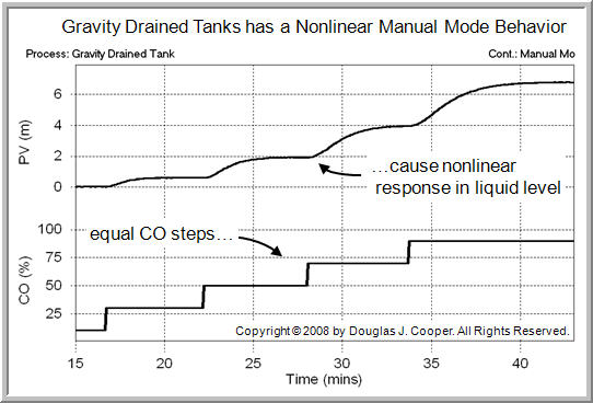
As shown, the CO is stepped in equal increments, yet the response (and thus the Kp,Tp, and/or Өp) changes as the level in the tank rises.
We address this concern by specifying a design level of operation (DLO) as the first step of our controller design and tuning recipe. If we are careful about how and where we collect our test data, we heighten the probability that the recipe will yield a controller with our desired performance.
The DLO includes where we expect the set point, SP, and measured process variable, PV, to be during normal operation, and the range of values the SP and PV might assume so we can explore the nature of the process across that range.
For the gravity drained tanks, the PV is liquid level in the lower tank. For this control study, we choose:
- Design PV and SP = 2.2 m with range of 2.0 to 2.4 m
The DLO also considers our major disturbances. We should know the normal or typical values for our major disturbances and be reasonably confident that they are quiet so we may proceed with a dynamic (bump) test.
The gravity drained tanks process has one major disturbance variable, the pumped flow disturbance, D. For this study, D is normally steady at about 2 L/min, but certain operations in the plant cause it to momentarily spike up to 5 L/min for brief periods.
Rejecting this disturbance is a major objective in our controller design. For this study, then:
- Design D = 2 L/min with occasional spikes up to 5 L/min
Step 2: Collect Data at the DLO (Design Level of Operation)
The next step in our recipe is to collect dynamic process data as near as practical to our design level of operation. We do this with a bump test, where we step or pulse the CO and collect data as the PV responds.
It is important to wait until the CO, PV and D have settled out and are as near to constant values as is possible for our particular operation before we start a bump test. The point of bumping a process is to learn about the cause and effect relationship between the CO and PV.
With the process steady, we are starting with a clean slate and as the PV responds to the CO bumps, the dynamic cause and effect behavior is isolated and evident in the data. On a practical note, be sure the data capture routine is enabled before the initial bump so all relevant data is collected.
While closed loop testing is an option, here we consider two open loop (manual mode) methods: the step test and the doublet test.
For either method, the CO must be moved far enough and fast enough to force a response in the PV that dominates the measurement noise.
Also, our bump should move the PV both above and below the DLO during testing. With data from each side of the DLO, the FOPDT model will be able to average out the nonlinear effects.
- Step Test
To collect data that will “average out” to our design level of operation, we start the test with the PV on one side of (either above or below) the DLO. Then, we step the CO so that the measurement moves across to settle on the other side of the DLO.
We acknowledge that it may be unrealistic to attempt such a precise step test in some production environments. But we should understand why we propose this ideal approach (answer: to average nonlinear process effects).
Recall that our DLO is a PV = 2.2 m and D = 2 L/min (though not shown on the plots, disturbance D remains constant at 2 L/min throughout the test).
Below, we set CO = 55% and the process steadies at a PV = 2.4 L.
Then, as shown below (click for a large view), we step the CO to 51% and the PV settles at abut 2.0 L/min. Thus, we have collected data “around” our design level of operation.
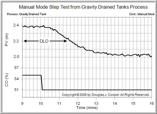
Note that we can start high and step the CO down (as above), or start low and step the CO up. Both methods produce dynamic data of equal value for our design and tuning recipe.
- Doublet Test
A doublet test, as shown below (click for a large view), is two CO pulses performed in rapid succession and in opposite direction.

The second pulse is implemented as soon as the process has shown a clear response to the first pulse that dominates the noise in the PV. It is not necessary to wait for the process to respond to steady state for either pulse.
The doublet test offers important benefits. Specifically, it:
- starts from and quickly returns to the design level of operation,
- produces data both above and below the design level to “average out” the nonlinear effects, and
- the PV always stays close to the DLO, thus minimizing off-spec production.
For these reasons, many industrial practitioners find the doublet to be the preferred method for generating open loop dynamic process data, though it does require that we use a commercial software tool for the model fitting task.
Modeling Process Dynamics
Next, we model the dynamics of the gravity drained tanks process and use the result in a series of control studies.
Graphical Modeling of Gravity Drained Tanks Step Test
We have explored the manual mode (open loop) operation and behavior of the gravity drained tanks process and have worked through the first two steps of the controller design and tuning recipe.
As those articles discuss:
- Our measured process variable, PV, is liquid level in the lower tank,
- The set point, SP, is held constant during normal production operation,
- Our primary control challenge is rejecting unexpected disruptions from D, the pumped flow disturbance.
We have generated process data from both a step test and a doublet test around our design level of operation (DLO), which for this study is:
- Design PV and SP = 2.2 m with range of 2.0 to 2.4 m
- Design D = 2 L/min with occasional spikes up to 5 L/min
Here we present step 3 of our recipe and focus on a graphical analysis of the step test data. Next we will explore modeling of the doublet test data using software.
Data Accuracy
We should understand that real plant data is rarely as perfect as that shown in the plots below. As such, we should not seek to extract more information from our data than it actually contains.
In the analyses presented here, we display extra decimals of accuracy only because we will be comparing different modeling methods over several articles. The extra accuracy will help when we make side-by-side comparisons of the results.
Step 3: Fit a FOPDT Model to the Data
The third step of the recipe is to describe the overall dynamic behavior of the process with an approximating first order plus dead time (FOPDT) dynamic model.
We will move quickly through the graphical analysis of step response data as we already presented details of the procedure in the heat exchanger study.
- Process Gain – The “Which Direction and How Far” Variable
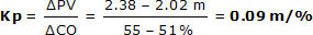
Process gain, Kp, describes how far the PV moves in response to a change in controller output (CO). It is computed: 
where ΔPV and ΔCO represent the total change from initial to final steady state. The path or length of time the PV takes to get to its new steady state does not enter into the Kp calculation.
Reading the numbers off of our step test plot below (click for a large view), the CO was stepped from a steady value of 55% down to 51%.
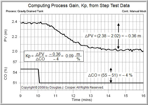
The PV was initially steady at 2.38 m, and in response to the CO step, moved down to a new steady value of 2.02 m.

Using these in the Kp equation above, the process gain for the gravity drained tanks process around a DLO (design level of operation) PV of about 2.2 m when the pumped disturbance (not shown in the plot) is constant at 2 L/min is:
For further discussion and details, another example of a process gain calculation from step test data for the heat exchanger is presented here.
- Time Constant – The “How Fast” Variable
The time constant, Tp, describes how fast the PV moves in response to a change in the CO.
For step test data, Tp can be computed as the time that passes from when the PV shows its first response to the CO step, until when the PV reaches 63% of the total ΔPV change that is going to occur.
The time constant must be positive and have units of time. For controllers used on processes comprised of gases, liquids, powders, slurries and melts, Tp most often has units of minutes or seconds.
For step test data, we compute Tp in five steps (see plot below):
1. Determine ΔPV, the total change in PV from final steady state minus initial steady state
2. Compute the value of the PV that is 63% of the way toward the total ΔPV change, or “initial steady state + 0.63(ΔPV)”
3. Note the time when the PV passes through the “initial steady state + 0.63(ΔPV)” value
4. Subtract from it the time when the “PV starts a first clear response” to the step change in the CO
5. The passage of time from step 4 minus step 3 is the process time constant, Tp.
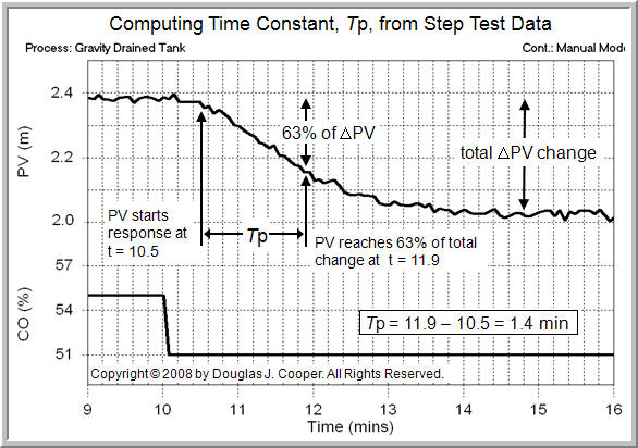
| 1. | The PV was initially steady at 2.38 m and moved to a final steady state of 2.02m. The total change, ΔPV, is “final minus initial steady state” or: ΔPV = 2.02 – 2.38 = –0.36 m |
| 2. | The value of the PV that is 63% of the way toward this total change is “initial steady state + 0.63(ΔPV)” or: Initial PV + 0.63(ΔPV) = 2.38 + 0.63(–0.36) = 2.38 – 0.23 = 2.15 m |
| 3. | The time when the PV passes through the “initial steady state PV + 0.63(ΔPV)” point of 2.15 m is: Time to 0.63(ΔPV) = Time to 2.15 = 11.9 min |
| 4. | The time when the “PV starts a first response” to the CO step is: Time PV response starts = 10.5 min |
| 5. | The time constant is “time to 63%(ΔPV)” minus “time PV response starts” or: Tp = 11.9 – 10.5 = 1.4 min |
There are further details and discussion on the process time constant and its calculation from step test data in the heat exchanger example presented in another article.
- Dead Time – The “How Much Delay” Variable
Dead time, Өp, is the time delay that passes from when a CO action is made and the measured PV shows its first clear response to that action.
Like a time constant, dead time has units of time, must always be positive, and for processes with streams comprised of gasses, liquids, powders, slurries and melts, is most often expressed in minutes or seconds.
Estimating dead time, Өp, from step test data is a three step procedure:
1. Locate the time when the “PV starts a first clear response” to the step change in the CO. We already identified this point when we computed Tp above.
2. Locate the point in time when the CO was stepped from its original value to its new value.
3. Dead time, Өp, is the difference in time of step 1 minus step 2.

Applying this procedure to the step test plot above (click for a large view):
| 1. | As identified in the plot above, the PV starts a first clear response to the CO step at 10.5 min (this is the same point we identified in the Tp analysis), |
| 2. | The CO step occurred at 10.0 min, and thus, |
| 3. |
Өp = 10.0 – 10.5 = 0.5 min |
Additional details and discussion on process dead time and its calculation from step test data can be found in the heat exchanger example presented here.
Note on Units
During a dynamic analysis study, it is best practice to express Tp and Өp in the same units (e.g. both in minutes or both in seconds). The tuning correlations and design rules assume consistent units.
Also, the process gain, Kp, should be expressed in the same (though inverse) units of the controller gain, Kc, (or proportional band, PB) used by our manufacturer.
Control is challenging enough without adding computational error to our problems.
Validating Our FOPDT Model
It is good practice to validate our FOPDT model before proceeding with design and tuning. If our model describes the dynamic data, and the data is reflective of the process behavior, then the last step of the recipe follows smoothly.
The FOPDT model parameters we computed from the analysis of the step test data are:
- Process gain (how far), Kp = 0.09 m/%
- Time constant (how fast), Tp = 1.4 min
- Dead time (how much delay), Өp = 0.5 min
Recall that, using the nomenclature of this site, the FOPDT dynamic model has the general form:
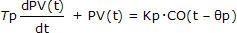
And this means that the dynamic behavior of the gravity drained tanks can be reasonably approximated around our DLO as:
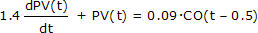
Where: t [=] min, PV(t) [=] m, CO(t − Өp)[=] %
The plot below (click for large view) compares step test data from the gravity drained tanks process to this FOPDT model.
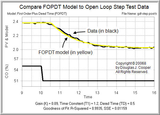
Visual inspection confirms that the simple FOPDT model provides a very good approximation for the behavior of this process.
Specifically, our graphical analysis tells us that for the gravity drained tanks process, with a DLO PV of about 2.2 m when the pumped disturbance is constant at 2 L/min:
- the direction PV moves given a change in CO
- how far PV ultimately travels for a given change in CO
- How fast PV moves as it heads toward its new steady state
- how much delay occurs between when CO changes and PV first begins to respond
This is precisely the information we need to proceed with confidence to step 4 of the design and tuning recipe.
Modeling Doublet Test Data
We had suggested in a previous article that a doublet test offers benefits as an open loop method for generating dynamic process data. These include that the process:
| starts from and quickly returns to the DLO, | |
| yields data both above and below the design level to “average out” the nonlinear effects, and | |
| the PV always stays close to the DLO, thus minimizing off-spec production. |
We explore using commercial software to fit a FOPDT model to doublet test data for the gravity drained tanks in this article.
Modeling Gravity Drained Tanks Data Using Software
Design Level of Operation for the Jacketed Stirred Reactor Process
Modeling the Dynamics of the Jacketed Stirred Reactor with Software
Exploring the FOPDT Model With a Parameter Sensitivity Study
Design and Tuning Recipe Must Consider Nonlinear Process Behavior
A Controller’s “Process” Goes From Wire Out to Wire In
The Normal or Standard PID Algorithm
The P-Only Control Algorithm
P-Only Control of the Heat Exchanger Shows Offset
P-Only Disturbance Rejection Of The Gravity Drained Tanks
Controller Gain Is Dimensionless in Commercial Systems

 浙公网安备 33010602011771号
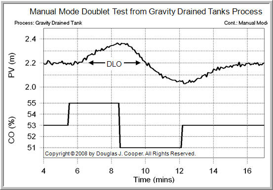
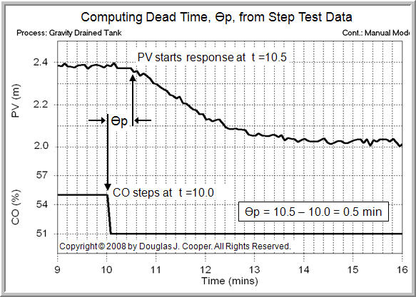