数据可视化
数据可视化
EDA探索性数据分析exploded data analysis
主要介绍工具的使用
matplotlib、seaborn
BI business information
集成工具
Power BI
Tableau
Fine BI
Metabase
superset
代码工具
Matplotlib
seaborn
pyecharts
echarts
HTML/Javascript
Flask,轻代码工具,微框架
画各种图
导入包
import matplotlib.pyplot as plt
import seaborn as sns
import numpy as np
import pandas as pd
import os
from matplotlib.font_manager import FontProperties
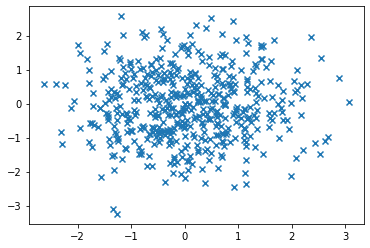
散点图
def scatter():
#数据准备
N = 500;
x = np.random.randn(N);
y = np.random.randn(N);
#用matplotlib画
plt.scatter(x,y,marker='x');
plt.show();
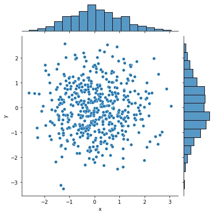
#用seaborn画
df = pd.DataFrame({'x':x,'y':y})
sns.jointplot(x="x",y="y",data=df,kind='scatter')
plt.show()
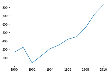
折线图
def line_chart():
#数据准备
x = [1900, 1901, 1902, 1903, 1904, 1905, 1906, 1907, 1908, 1909, 1910]
y = [265, 323, 136, 220, 305, 350, 419, 450, 560, 720, 830]
#使用matplotlib
plt.plot(x,y)
plt.show()
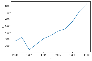
#使用seaborn
df = pd.DataFrame({'x':x,'y':y})
sns.lineplot(x="x",y="y",data=df)
plt.show()
条形图
def bar_chart():
    # 数据准备
	x = ['c1', 'c2', 'c3', 'c4']
	y = [15, 18, 5, 26]
	# 用Matplotlib画条形图
	plt.bar(x, y)
	plt.show()
	# 用Seaborn画条形图
	sns.barplot(x, y)
	plt.show()
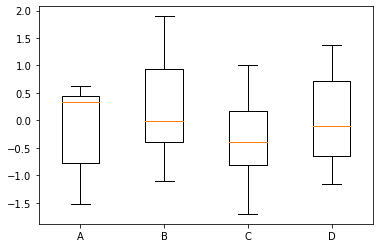
箱线图
def box_plots():
	# 数据准备
	# 生成0-1之间的20*4维度数据
	data=np.random.normal(size=(10,4))
	lables = ['A','B','C','D']
	# 用Matplotlib画箱线图
	plt.boxplot(data,labels=lables)
	plt.show()
	# 用Seaborn画箱线图
	df = pd.DataFrame(data, columns=lables)
	sns.boxplot(data=df)
	plt.show()

饼图
# 饼图1
def pie_chart():
	# 数据准备
	nums = [25, 33, 37]
	# 射手adc:法师apc:坦克tk
	labels = ['ADC','APC', 'TK']
	# 用Matplotlib画饼图
	plt.pie(x = nums, labels=labels)
	plt.show()

# 饼图2
def pie_chart2():
	# 数据准备
	data = {}
	data['ADC'] = 25
	data['APC'] = 33
	data['TK'] = 37
	data = pd.Series(data)
	data.plot(kind = "pie", label='heros')
	plt.show()
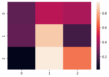
热力图
def thermodynamic():
	# 数据准备
	np.random.seed(33)
	data = np.random.rand(3, 3)
	print(data)
	heatmap = sns.heatmap(data)
	plt.show()
蜘蛛图
def spider_chart():
	# 数据准备
	labels=np.array([u"推进","KDA",u"生存",u"团战",u"发育",u"输出"])
	stats=[76, 58, 67, 97, 86, 58]
	# 画图数据准备,角度、状态值
	angles=np.linspace(0, 2*np.pi, len(labels), endpoint=False)
	stats=np.concatenate((stats,[stats[0]]))
	angles=np.concatenate((angles,[angles[0]]))
	# 用Matplotlib画蜘蛛图
	fig = plt.figure()
	ax = fig.add_subplot(111, polar=True)
	ax.plot(angles, stats, 'o-', linewidth=2)
	ax.fill(angles, stats, alpha=0.25)
	# 设置中文字体
	font = FontProperties(fname=r"./simhei.ttf", size=14)
	ax.set_thetagrids(angles * 180/np.pi, labels, FontProperties=font)
	plt.show()
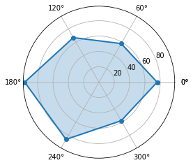
注释:这个图片中文没设置好,所以和代码实际想要展示的内容有些许出入
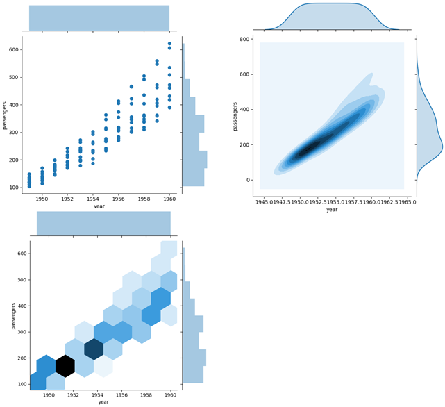
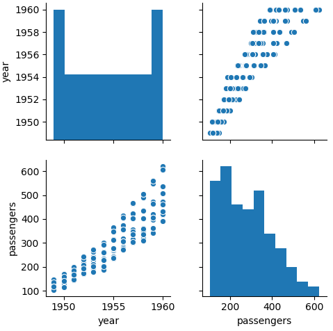
二元变量分布图
def jointplot():
# 数据准备
flights = sns.load_dataset("flights")
# 用Seaborn画二元变量分布图(散点图,核密度图,Hexbin图)
sns.jointplot(x="year", y="passengers", data=flights, kind='scatter')
sns.jointplot(x="year", y="passengers", data=flights, kind='kde')
sns.jointplot(x="year", y="passengers", data=flights, kind='hex')
plt.show()#数据集没找到,加载不出来画不出图,直接引用PPT上的图了
成对关系图
def pairplot():
# 数据准备	flights = sns.load_dataset('flights')	# 用Seaborn画成对关系	sns.pairplot(flights)	plt.show()
热力图
def thermodynamic2():
flights = sns.load_dataset('flights')
print(flights)	flights=flights.pivot('month','year','passengers')
#pivot函数重要
print(flights)	sns.heatmap(flights)
#注意这里是直接传入数据集即可,不需要再单独传入x和y了
sns.heatmap(flights,linewidth=.5,annot=True,fmt='d')
plt.show()
词云图
from wordcloud import WordCloud
import pandas as pd
import matplotlib.pyplot as plt
from PIL import Image
import numpy as npfrom lxml
import etreefrom nltk.tokenize
import word_tokenize
import jieba
# 去掉停用词
def remove_stop_words(f):
stop_words = ['Movie', 'The']
for stop_word in stop_words:
f = f.replace(stop_word, '')
return f
# 生成词云def create_word_cloud(f):
print('根据词频,开始生成词云!')
f = remove_stop_words(f)
# 使用NLTK进行分词
cut_text = word_tokenize(f)
#print(cut_text)
cut_text = " ".join(cut_text)
wc = WordCloud(		max_words=100,		width=2000,		height=1200,    )
# 将需要进行词云展示的文字
wordcloud = wc.generate(cut_text)
# 写词云图片
wordcloud.to_file("wordcloud.jpg")
# 显示词云文件
plt.imshow(wordcloud)
plt.axis("off")	plt.show()
# 数据加载
data = pd.read_csv('./Market_Basket_Optimisation.csv', header=None)
print(data.shape)
# 将数据放到transactions中
transactions = []
# 存储key:value
item_count = {}
for i in range(0, data.shape[0]):
for j in range(20):
item = str(data.values[i,j])
# 当item不为空的时候
if item != 'nan':
if item not in item_count:
item_count[item] = 1
else:
item_count[item] += 1
transactions.append(item)# 生成词云all_word = ' '.join(x for x in transactions)
#print(all_word)create_word_cloud(all_word)
# 输出Top10商品, reverse=True 代表降序
print(sorted(item_count.items(), key=lambda x:x[1], reverse=True))
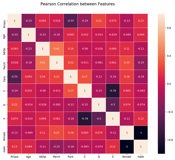
决策树可视化
# 决策树可视化import pydotplusfrom sklearn.externals.six import StringIOfrom sklearn.tree import export_graphvizdef show_tree(clf): dot_data = StringIO() export_graphviz(clf, out_file=dot_data) graph = pydotplus.graph_from_dot_data(dot_data.getvalue()) graph.write_pdf("titanic_tree.pdf")

 浙公网安备 33010602011771号