全卷积网络FCN

全卷积网络FCN

fcn是深度学习用于图像分割的鼻祖.后续的很多网络结构都是在此基础上演进而来.

图像分割即像素级别的分类.

语义分割的基本框架:
前端fcn(以及在此基础上的segnet,deconvnet,deeplab等) + 后端crf/mrf

FCN是分割网络的鼻祖,后面的很多网络都是在此基础上提出的.
论文地址

和传统的分类网络相比,就是将传统分类网络的全连接层用反卷积层替代.得到一个和图像大小一致的feature map。本篇文章用的网络是VGG.

主要关注两点

• 全连接层替换成卷积层.用反卷积的方式完成上采样
• 不同layer的输出要做相加.用以增强feature map的表达能力.

反卷积(deconvolutional)

关于反卷积(也叫转置卷积)的详细推导,可以参考:<https://blog.csdn.net/LoseInVain/article/details/81098502＞

简单滴说就是:卷积的反向操作．以4x4矩阵Ａ为例,卷积核Ｃ(3x3,stride=1),通过卷积操作得到一个2x2的矩阵B. 转置卷积即已知B,要得到A,我们要找到卷积核C,使得B相当于A通过C做正向卷积,得到B.

转置卷积是一种上采样的方法.

跳连(skip layer)

如果只用特征提取部分(也就是VGG全连接层之前的部分)得到的feature map做上采样将feature map还原到图像输入的size的话,feature不够精确.所以采用不同layer的feature map做上采样再组合起来.

代码解析

源码:https://github.com/pochih/FCN-pytorch

其中的核心代码如下:

class FCNs(nn.Module):

    def __init__(self, pretrained_net, n_class):
        super().__init__()
        self.n_class = n_class
        self.pretrained_net = pretrained_net
        self.relu    = nn.ReLU(inplace=True)
        self.deconv1 = nn.ConvTranspose2d(512, 512, kernel_size=3, stride=2, padding=1, dilation=1, output_padding=1)
        self.bn1     = nn.BatchNorm2d(512)
        self.deconv2 = nn.ConvTranspose2d(512, 256, kernel_size=3, stride=2, padding=1, dilation=1, output_padding=1)
        self.bn2     = nn.BatchNorm2d(256)
        self.deconv3 = nn.ConvTranspose2d(256, 128, kernel_size=3, stride=2, padding=1, dilation=1, output_padding=1)
        self.bn3     = nn.BatchNorm2d(128)
        self.deconv4 = nn.ConvTranspose2d(128, 64, kernel_size=3, stride=2, padding=1, dilation=1, output_padding=1)
        self.bn4     = nn.BatchNorm2d(64)
        self.deconv5 = nn.ConvTranspose2d(64, 32, kernel_size=3, stride=2, padding=1, dilation=1, output_padding=1)
        self.bn5     = nn.BatchNorm2d(32)
        self.classifier = nn.Conv2d(32, n_class, kernel_size=1)

    def forward(self, x):
        output = self.pretrained_net(x)
        x5 = output['x5']  # size=(N, 512, x.H/32, x.W/32)
        x4 = output['x4']  # size=(N, 512, x.H/16, x.W/16)
        x3 = output['x3']  # size=(N, 256, x.H/8,  x.W/8)
        x2 = output['x2']  # size=(N, 128, x.H/4,  x.W/4)
        x1 = output['x1']  # size=(N, 64, x.H/2,  x.W/2)

        score = self.bn1(self.relu(self.deconv1(x5)))     # size=(N, 512, x.H/16, x.W/16)
        score = score + x4                                # element-wise add, size=(N, 512, x.H/16, x.W/16)
        score = self.bn2(self.relu(self.deconv2(score)))  # size=(N, 256, x.H/8, x.W/8)
        score = score + x3                                # element-wise add, size=(N, 256, x.H/8, x.W/8)
        score = self.bn3(self.relu(self.deconv3(score)))  # size=(N, 128, x.H/4, x.W/4)
        score = score + x2                                # element-wise add, size=(N, 128, x.H/4, x.W/4)
        score = self.bn4(self.relu(self.deconv4(score)))  # size=(N, 64, x.H/2, x.W/2)
        score = score + x1                                # element-wise add, size=(N, 64, x.H/2, x.W/2)
        score = self.bn5(self.relu(self.deconv5(score)))  # size=(N, 32, x.H, x.W)
        score = self.classifier(score)                    # size=(N, n_class, x.H/1, x.W/1)

        return score  # size=(N, n_class, x.H/1, x.W/1)

train.py中

vgg_model = VGGNet(requires_grad=True, remove_fc=True)
fcn_model = FCNs(pretrained_net=vgg_model, n_class=n_class)

这里我们重点看FCN的forward函数

    def forward(self, x):
        output = self.pretrained_net(x)
        x5 = output['x5']  # size=(N, 512, x.H/32, x.W/32)
        x4 = output['x4']  # size=(N, 512, x.H/16, x.W/16)
        x3 = output['x3']  # size=(N, 256, x.H/8,  x.W/8)
        x2 = output['x2']  # size=(N, 128, x.H/4,  x.W/4)
        x1 = output['x1']  # size=(N, 64, x.H/2,  x.W/2)

        score = self.bn1(self.relu(self.deconv1(x5)))     # size=(N, 512, x.H/16, x.W/16)
        score = score + x4                                # element-wise add, size=(N, 512, x.H/16, x.W/16)
        score = self.bn2(self.relu(self.deconv2(score)))  # size=(N, 256, x.H/8, x.W/8)
        score = score + x3                                # element-wise add, size=(N, 256, x.H/8, x.W/8)
        score = self.bn3(self.relu(self.deconv3(score)))  # size=(N, 128, x.H/4, x.W/4)
        score = score + x2                                # element-wise add, size=(N, 128, x.H/4, x.W/4)
        score = self.bn4(self.relu(self.deconv4(score)))  # size=(N, 64, x.H/2, x.W/2)
        score = score + x1                                # element-wise add, size=(N, 64, x.H/2, x.W/2)
        score = self.bn5(self.relu(self.deconv5(score)))  # size=(N, 32, x.H, x.W)
        score = self.classifier(score)                    # size=(N, n_class, x.H/1, x.W/1)

        return score  # size=(N, n_class, x.H/1, x.W/1)

可见FCN的输入为(batch_size,c,h,w),输出为(batch_size,class,h,w).
首先是经过vgg的特征提取层,可以得到feature map. 5个max_pool后的feature map的size分别为

        x5 = output['x5']  # size=(N, 512, x.H/32, x.W/32)
        x4 = output['x4']  # size=(N, 512, x.H/16, x.W/16)
        x3 = output['x3']  # size=(N, 256, x.H/8,  x.W/8)
        x2 = output['x2']  # size=(N, 128, x.H/4,  x.W/4)
        x1 = output['x1']  # size=(N, 64, x.H/2,  x.W/2)

之后每一个pool layer的feature map都经过一次2倍上采样,并与前一个pool layer的输出进行element-wise add.(resnet也有类似操作).从而使得上采样后的feature map信息更充分更精准,模型的鲁棒性会更好.
例如以输入图片尺寸为224x224为例,pool4的输出为(,512,14,14),pool5的输出为(,512,7,7),反卷积后得到(,512,14,14),再与pool4的输出做element-wise add。得到的仍然是(,512,14,14). 对这个输出做上采样得到(,256,28,28)再与pool3的输出相加. 依次类推,最终得到(,64,112,112).

此后,再做一次反卷积上采样得到(,32,224,224),之后卷积得到(,n_class,224,224)。即得到n_class张224x224的feature map。

下图显示了随着上采样的进行,得到的feature map细节越来越丰富.

损失函数

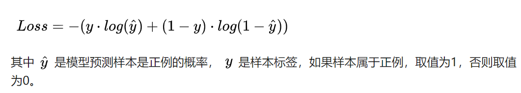
criterion = nn.BCEWithLogitsLoss()

损失函数采用二分类交叉熵.torch中有2个计算二分类交叉熵的函数

• BCELoss()
• BCEWithLogitsLoss()

后者只是在前者的基础上,对输入先做一个sigmoid将输入转换到0-1之间.即BCEWithLogitsLoss = Sigmoid + BCELoss

一个具体的例子可以参考:https://blog.csdn.net/qq_22210253/article/details/85222093