从头学pytorch(十五):AlexNet

AlexNet

AlexNet是2012年提出的一个模型,并且赢得了ImageNet图像识别挑战赛的冠军.首次证明了由计算机自动学习到的特征可以超越手工设计的特征,对计算机视觉的研究有着极其重要的意义.

AlexNet的设计思路和LeNet是非常类似的.不同点主要有以下几点:

激活函数由sigmoid改为Relu
AlexNet使用了dropout,LeNet没有使用
AlexNet引入了大量的图像增广，如翻转、裁剪和颜色变化，从而进一步扩大数据集来缓解过拟合

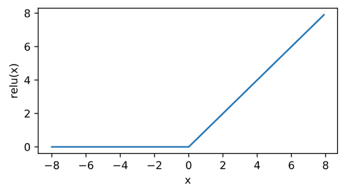
激活函数

relu

\[\text{ReLU}(x) = \max(x, 0). \]

其曲线及导数的曲线图绘制如下:

sigmoid

其曲线及导数的曲线图绘制如下:

\[\text{sigmoid}(x) = \frac{1}{1 + \exp(-x)}. \]

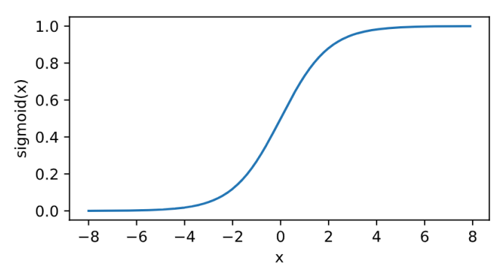
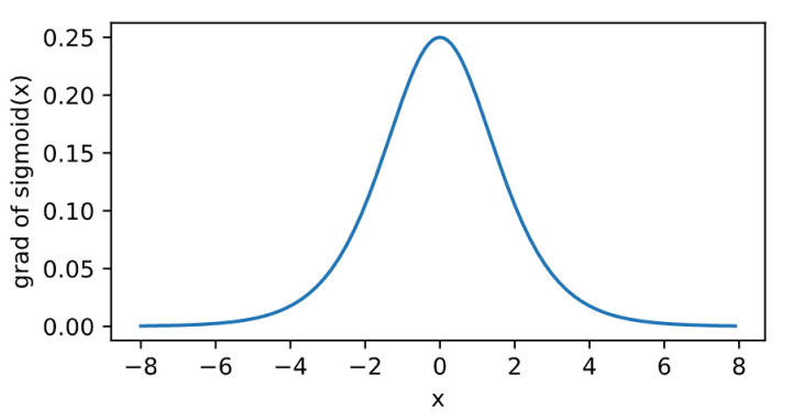
relu的好处主要有两点：

计算更简单,没有了指数运算
在正数区间,梯度恒定为1,而sigmoid在接近0和1时,梯度几乎为0,会导致模型参数更新极为缓慢

现在大多模型激活函数都选择Relu了.

模型结构

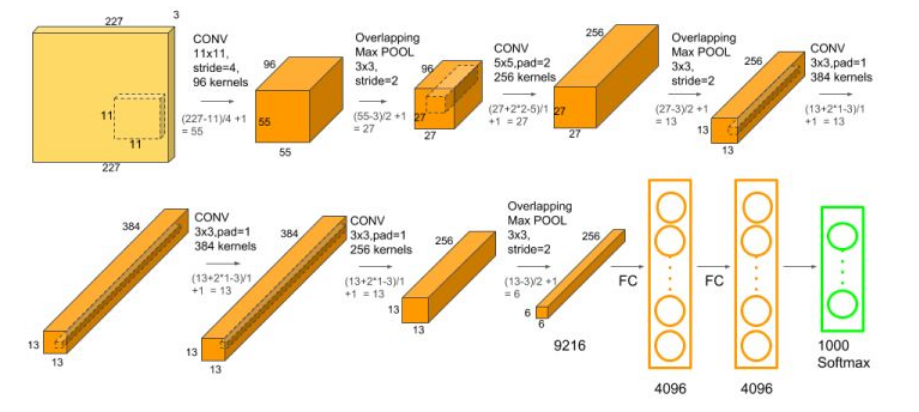
AlexNet结构如下:

早期的硬件设备计算能力不足,所以上面的图分成了两部分,把不同部分的计算分散到不同的gpu上去,现在已经完全没有这种必要了.比如第一个卷积层的channel是48 x 2 = 96个.

细化的结构图:

根据上图,我们来写模型的定义:
首先,用一个11 x 11的卷积核,对224 x 224的输入,卷积后得到55 x 55 x　96的输出.
由于我们的图片是单通道的,那么我们有代码:

nn.Conv2d(1, 96, kernel_size=11, stride=4)

然而,我们测试一下他的输出.

X=torch.randn((1,1,224,224)) #batch x c x h x w
net = nn.Conv2d(1, 96, kernel_size=11, stride=4)
out = net(X)
print(out.shape)

输出

torch.Size([1, 96, 54, 54])

我们将代码修改为

nn.Conv2d(3, 64, kernel_size=11, stride=4, padding=2)

再用相同的代码测试输出

X=torch.randn((1,1,224,224)) #batch x c x h x w
net = nn.Conv2d(1, 96, kernel_size=11, stride=4,padding=2)
out = net(X)
print(out.shape)

输出

torch.Size([1, 96, 55, 55])

由此可见,第一个卷积层的实现应该是

nn.Conv2d(3, 64, kernel_size=11, stride=4, padding=2)

搜索pytorch的padding策略,https://blog.csdn.net/g11d111/article/details/82665265基本都是抄这篇的,这篇里指出

　显然，padding=1的效果是：原来的输入层基础上，上下左右各补了一行！

然而实测和文章中的描述不一致.

net = nn.Conv2d(1, 1, 3,padding=0)
X= torch.randn((1,1,5,5))
print(X)
out=net(X)
print(out)

net2 = nn.Conv2d(1, 1, 3,padding=1)
out=net(X)
print(out)

输出

tensor([[[[-2.3052,  0.7220,  0.3106,  0.0605, -0.8304],
          [-0.0831,  0.0168, -0.9227,  2.2891,  0.6738],
          [-0.7871, -0.2234, -0.2356,  0.2500,  0.8389],
          [ 0.7070,  1.1909,  0.2963, -0.7580,  0.1535],
          [ 1.0306, -1.1829,  3.1201,  1.0544,  0.3521]]]])
tensor([[[[-0.1129,  0.7711, -0.6452],
          [-0.3387,  0.1025,  0.3039],
          [ 0.1604,  0.2709,  0.0740]]]], grad_fn=<MkldnnConvolutionBackward>)
tensor([[[[-0.1129,  0.7711, -0.6452],
          [-0.3387,  0.1025,  0.3039],
          [ 0.1604,  0.2709,  0.0740]]]], grad_fn=<MkldnnConvolutionBackward>)

到目前,我也没有把torch的padding策略搞清楚.知道的同学请评论留言.我的torch版本是1.2.0

AlexNet的激活函数采用的是Relu,所以

nn.ReLU(inplace=True)

接下来用一个3 x 3的卷积核去做最大池化,步幅为2,得到[27,27,96]的输出

nn.MaxPool2d(kernel_size=3, stride=2)

我们测试一下:

X=torch.randn((1,1,224,224)) #batch x c x h x w
net = nn.Sequential(
    nn.Conv2d(1, 96, kernel_size=11, stride=4,padding=2),
    nn.ReLU(),
    nn.MaxPool2d(kernel_size=3,stride=2)
)
out = net(X)
print(out.shape)

输出

torch.Size([1, 96, 27, 27])

至此,一个基本的卷积单元的定义就完成了,包括卷积,激活,池化．类似的,我们可以写出后续各层的定义.

AlexNet有5个卷积层,第一个卷积层的卷积核大小为11x11,第二个卷积层的卷积核大小为5x5,其余的卷积核均为3x3.第一二五个卷积层后做了最大池化操作,窗口大小为3x3,步幅为2.

这样,卷积层的部分如下:

net = nn.Sequential(
    nn.Conv2d(1, 96, kernel_size=11, stride=4,padding=2), #[1,96,55,55] order:batch,channel,h,w
    nn.ReLU(),
    nn.MaxPool2d(kernel_size=3,stride=2),                 #[1,96,27,27]

    nn.Conv2d(96, 256, kernel_size=5, stride=1,padding=2),#[1,256,27,27]
    nn.ReLU(),
    nn.MaxPool2d(kernel_size=3,stride=2),                 #[1,256,13,13]

    nn.Conv2d(256, 384, kernel_size=3, stride=1,padding=1), #[1,384,13,13]
    nn.ReLU(),

    nn.Conv2d(384, 384, kernel_size=3, stride=1,padding=1), #[1,384,13,13]
    nn.ReLU(),

    nn.Conv2d(384, 256, kernel_size=3, stride=1,padding=1), #[1,256,13,13]
    nn.ReLU(),
    nn.MaxPool2d(kernel_size=3,stride=2),       #[1,256,6,6]
)

接下来是全连接层的部分:

net = nn.Sequential(
    nn.Linear(256*6*6,4096),
    nn.ReLU(),
    nn.Dropout(0.5),　　#dropout防止过拟合
    nn.Linear(4096,4096),
    nn.ReLU(),
    nn.Dropout(0.5),　　#dropout防止过拟合
    nn.Linear(4096,10) #我们最终要10分类
)

全连接层的参数数量过多,为了防止过拟合,我们在激活层后面加入了dropout层．

这样的话我们就可以给出模型定义:

class AlexNet(nn.Module):
    def __init__(self):
        super(AlexNet, self).__init__()
        self.conv = nn.Sequential(  
            nn.Conv2d(1, 96, kernel_size=11, stride=4, padding=2), # [1,96,55,55] order:batch,channel,h,w
            nn.ReLU(),
            nn.MaxPool2d(kernel_size=3, stride=2),  # [1,96,27,27]

            nn.Conv2d(96, 256, kernel_size=5, stride=1,padding=2),  # [1,256,27,27]
            nn.ReLU(),
            nn.MaxPool2d(kernel_size=3, stride=2),  # [1,256,13,13]

            nn.Conv2d(256, 384, kernel_size=3, stride=1,padding=1),  # [1,384,13,13]
            nn.ReLU(),

            nn.Conv2d(384, 384, kernel_size=3, stride=1,padding=1),  # [1,384,13,13]
            nn.ReLU(),

            nn.Conv2d(384, 256, kernel_size=3, stride=1,padding=1),  # [1,256,13,13]
            nn.ReLU(),
            nn.MaxPool2d(kernel_size=3, stride=2),  # [1,256,6,6]
        )

        self.fc = nn.Sequential(
            nn.Linear(256*6*6, 4096),
            nn.ReLU(),
            nn.Dropout(0.5),  # dropout防止过拟合
            nn.Linear(4096, 4096),
            nn.ReLU(),
            nn.Dropout(0.5),  # dropout防止过拟合
            nn.Linear(4096, 10)  # 我们最终要10分类
        )
    
    def forward(self, img):
        feature = self.conv(img) 
        output = self.fc(feature.view(img.shape[0], -1))#输入全连接层之前,将特征展平
        return output

加载数据

batch_size,num_workers=32,4
train_iter,test_iter = learntorch_utils.load_data(batch_size,num_workers,resize=224)

其中load_data定义于learntorch_utils.py．

def load_data(batch_size,num_workers,resize):
    trans = []
    if resize:
        trans.append(torchvision.transforms.Resize(size=resize))
    trans.append(torchvision.transforms.ToTensor())
    transform = torchvision.transforms.Compose(trans)

    mnist_train = torchvision.datasets.FashionMNIST(root='/home/sc/disk/keepgoing/learn_pytorch/Datasets/FashionMNIST',
                                                    train=True, download=True,
                                                    transform=transform)
    mnist_test = torchvision.datasets.FashionMNIST(root='/home/sc/disk/keepgoing/learn_pytorch/Datasets/FashionMNIST',
                                                train=False, download=True,
                                                transform=transform)

    train_iter = torch.utils.data.DataLoader(
        mnist_train, batch_size=batch_size, shuffle=True, num_workers=num_workers)
    test_iter = torch.utils.data.DataLoader(
        mnist_test, batch_size=batch_size, shuffle=False, num_workers=num_workers)
    
    return train_iter,test_iter

这里,构造了一个transform.对图像做一次resize.

    if resize:
        trans.append(torchvision.transforms.Resize(size=resize))
    trans.append(torchvision.transforms.ToTensor())
    transform = torchvision.transforms.Compose(trans)

定义模型

net = AlexNet().cuda()

由于全连接层的存在,AlexNet的参数还是非常多的.所以我们使用GPU做运算

定义损失函数

loss = nn.CrossEntropyLoss()

定义优化器

opt = torch.optim.Adam(net.parameters(),lr=0.01)

定义评估函数

def test():
    acc_sum = 0
    batch = 0
    for X,y in test_iter:
        X,y = X.cuda(),y.cuda()
        y_hat = net(X)
        acc_sum += (y_hat.argmax(dim=1) == y).float().sum().item()
        batch += 1
    print('acc_sum %d,batch %d' % (acc_sum,batch))

    return 1.0*acc_sum/(batch*batch_size)

验证在测试集上的准确率.

训练

num_epochs = 3
def train():
    for epoch in range(num_epochs):
        train_l_sum,batch = 0,0
        start = time.time()
        for X,y in train_iter:
            X,y = X.cuda(),y.cuda()
            y_hat = net(X)
            l = loss(y_hat,y)
            opt.zero_grad()
            l.backward()

            opt.step()
            train_l_sum += l.item()

            batch += 1
        test_acc = test()
        end = time.time()
        time_per_epoch =  end - start
        print('epoch %d,train_loss %f,test_acc %f,time %f' % 
                (epoch + 1,train_l_sum/(batch*batch_size),test_acc,time_per_epoch))

train()

输出

acc_sum 6297,batch 313
epoch 1,train_loss 54.029241,test_acc 0.628694,time 238.983008
acc_sum 980,batch 313
epoch 2,train_loss 0.106785,test_acc 0.097843,time 239.722055
acc_sum 1000,batch 313
epoch 3,train_loss 0.071997,test_acc 0.099840,time 239.459902

明显出现了过拟合.我们把学习率调整为0.001后,把batch_size调整为128

opt = torch.optim.Adam(net.parameters(),lr=0.001)

再训练,输出

acc_sum 8714,batch 79
epoch 1,train_loss 0.004351,test_acc 0.861748,time 156.573509
acc_sum 8813,batch 79
epoch 2,train_loss 0.002473,test_acc 0.871539,time 201.961380
acc_sum 8958,batch 79
epoch 3,train_loss 0.002159,test_acc 0.885878,time 202.349568

过拟合消失. 同时可以看到AlexNet由于参数过多,训练还是挺慢的.

posted @ 2020-01-08 18:29 core! 阅读(1342) 评论(0) 编辑收藏举报

会员力量，点亮园子希望

刷新页面返回顶部