
相关性系数及其python实现
参考文献:
1.python 皮尔森相关系数 https://www.cnblogs.com/lxnz/p/7098954.html
2.统计学之三大相关性系数(pearson、spearman、kendall) http://blog.sina.com.cn/s/blog_69e75efd0102wmd2.html
皮尔森系数
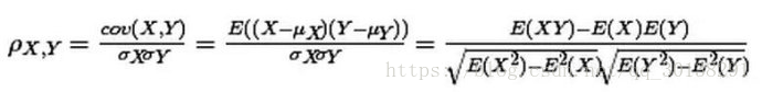
重点关注第一个等号后面的公式,最后面的是推导计算,暂时不用管它们。看到没有,两个变量(X, Y)的皮尔森相关性系数(ρX,Y)等于它们之间的协方差cov(X,Y)除以它们各自标准差的乘积(σX, σY)。
公式的分母是变量的标准差,这就意味着计算皮尔森相关性系数时,变量的标准差不能为0(分母不能为0),也就是说你的两个变量中任何一个的值不能都是相同的。如果没有变化,用皮尔森相关系数是没办法算出这个变量与另一个变量之间是不是有相关性的。
皮尔森相关系数(Pearson correlation coefficient)也称皮尔森积矩相关系数(Pearson product-moment correlation coefficient) ,是一种线性相关系数。皮尔森相关系数是用来反映两个变量线性相关程度的统计量。相关系数用r表示,其中n为样本量,分别为两个变量的观测值和均值。r描述的是两个变量间线性相关强弱的程度。r的绝对值越大表明相关性越强。
简单的相关系数的分类
0.8-1.0 极强相关
0.6-0.8 强相关
0.4-0.6 中等程度相关
0.2-0.4 弱相关
0.0-0.2 极弱相关或无相关
r描述的是两个变量间线性相关强弱的程度。r的取值在-1与+1之间,若r>0,表明两个变量是正相关,即一个变量的值越大,另一个变量的值也会越大;若r<0,表明两个变量是负相关,即一个变量的值越大另一个变量的值反而会越小。r 的绝对值越大表明相关性越强,要注意的是这里并不存在因果关系。
spearman correlation coefficient(斯皮尔曼相关性系数)
斯皮尔曼相关性系数,通常也叫斯皮尔曼秩相关系数。“秩”,可以理解成就是一种顺序或者排序,那么它就是根据原始数据的排序位置进行求解,这种表征形式就没有了求皮尔森相关性系数时那些限制。下面来看一下它的计算公式:
计算过程就是:首先对两个变量(X, Y)的数据进行排序,然后记下排序以后的位置(X’, Y’),(X’, Y’)的值就称为秩次,秩次的差值就是上面公式中的di,n就是变量中数据的个数,最后带入公式就可求解结果
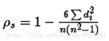
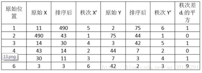
带入公式,求得斯皮尔曼相关性系数:ρs= 1-6*(1+1+1+9)/6*35=0.657
而且,即便在变量值没有变化的情况下,也不会出现像皮尔森系数那样分母为0而无法计算的情况。另外,即使出现异常值,由于异常值的秩次通常不会有明显的变化(比如过大或者过小,那要么排第一,要么排最后),所以对斯皮尔曼相关性系数的影响也非常小!
由于斯皮尔曼相关性系数没有那些数据条件要求,适用的范围就广多了。
kendall correlation coefficient(肯德尔相关性系数)
肯德尔相关性系数,又称肯德尔秩相关系数,它也是一种秩相关系数,不过它所计算的对象是分类变量。
分类变量可以理解成有类别的变量,可以分为
无序的,比如性别(男、女)、血型(A、B、O、AB);
有序的,比如肥胖等级(重度肥胖,中度肥胖、轻度肥胖、不肥胖)。
通常需要求相关性系数的都是有序分类变量。

Nc表示主客观评价值中一致的值的个数,Nd则表示了主观评估值和客观评估值不一样的个数
举个例子。比如评委对选手的评分(优、中、差等),我们想看两个(或者多个)评委对几位选手的评价标准是否一致;或者医院的尿糖化验报告,想检验各个医院对尿糖的化验结果是否一致,这时候就可以使用肯德尔相关性系数进行衡量。
pandas代码实现
pandas.DataFrame.corr()
DataFrame.corr(method='pearson', min_periods=1)[source]
Compute pairwise correlation of columns, excluding NA/null values
Parameters:
method : {‘pearson’, ‘kendall’, ‘spearman’}
pearson : standard correlation coefficient
kendall : Kendall Tau correlation coefficient
spearman : Spearman rank correlation
min_periods : int, optional
Minimum number of observations required per pair of columns to have a valid result. Currently only available for pearson and spearman correlation
Returns:y : DataFrame
import pandas as pd

df = pd.DataFrame({'A':[5,91,3],'B':[90,15,66],'C':[93,27,3]})

print(df.corr())

print(df.corr('spearman'))

print(df.corr('kendall'))

df2 = pd.DataFrame({'A':[7,93,5],'B':[88,13,64],'C':[93,27,3]})

print(df2.corr())

print(df2.corr('spearman'))

print(df2.corr('kendall'))
numpy代码实现
numpy.corrcoef(x,y = None,rowvar = True,bias = <class'numpy._globals._NoValue'>,ddof = <class'numpy._globals._NoValue'> )
返回Pearson乘积矩相关系数。
cov有关更多详细信息,请参阅文档。相关系数矩阵R和协方差矩阵C之间的关系为
R的值在-1和1之间(含)。
参数:
x:array_like
包含多个变量和观察值的1维或2维数组。x的每一行代表一个变量,每一列都是对所有这些变量的单独观察。另请参阅下面的rowvar。
y:array_like,可选
一组额外的变量和观察。y的形状与x相同。
rowvar:布尔,可选
如果rowvar为True(默认),则每行表示一个变量,并在列中有观察值。否则,该关系将被转置:每列表示一个变量,而行包含观察值。
bias : _NoValue, optional Has no effect, do not use. Deprecated since version 1.10.0.
ddof : _NoValue, optional Has no effect, do not use. Deprecated since version 1.10.0.
返回:
R:ndarray 变量的相关系数矩阵。
import numpy as np

vc=[1,2,39,0,8]

vb=[1,2,38,0,8]

print(np.mean(np.multiply((vc-np.mean(vc)),(vb-np.mean(vb))))/(np.std(vb)*np.std(vc)))

#corrcoef得到相关系数矩阵(向量的相似程度)

print(np.corrcoef(vc,vb))
Spearman’s Rank Correlation
Spearman’s rank correlation is named for Charles Spearman.
It may also be called Spearman’s correlation coefficient and is denoted by the lowercase greek letter rho (p). As such, it may be referred to as Spearman’s rho.
This statistical method quantifies the degree to which ranked variables are associated by a monotonic function, meaning an increasing or decreasing relationship. As a statistical hypothesis test, the method assumes that the samples are uncorrelated (fail to reject H0).
The Spearman rank-order correlation is a statistical procedure that is designed to measure the relationship between two variables on an ordinal scale of measurement.
— Page 124, Nonparametric Statistics for Non-Statisticians: A Step-by-Step Approach, 2009.
The intuition for the Spearman’s rank correlation is that it calculates a Pearson’s correlation (e.g. a parametric measure of correlation) using the rank values instead of the real values. Where the Pearson’s correlation is the calculation of the covariance (or expected difference of observations from the mean) between the two variables normalized by the variance or spread of both variables.
Spearman’s rank correlation can be calculated in Python using the spearmanr() SciPy function.
The function takes two real-valued samples as arguments and returns both the correlation coefficient in the range between -1 and 1 and the p-value for interpreting the significance of the coefficient.
|
1
2
|
# calculate spearman's correlation
coef, p = spearmanr(data1, data2)
|
We can demonstrate the Spearman’s rank correlation on the test dataset. We know that there is a strong association between the variables in the dataset and we would expect the Spearman’s test to find this association.
The complete example is listed below.
|
1
2
3
4
5
6
7
8
9
10
11
12
13
14
15
16
17
18
|
# calculate the spearman's correlation between two variables
from numpy.random import rand
from numpy.random import seed
from scipy.stats import spearmanr
# seed random number generator
seed(1)
# prepare data
data1 = rand(1000) * 20
data2 = data1 + (rand(1000) * 10)
# calculate spearman's correlation
coef, p = spearmanr(data1, data2)
print('Spearmans correlation coefficient: %.3f' % coef)
# interpret the significance
alpha = 0.05
if p > alpha:
print('Samples are uncorrelated (fail to reject H0) p=%.3f' % p)
else:
print('Samples are correlated (reject H0) p=%.3f' % p)
|
Running the example calculates the Spearman’s correlation coefficient between the two variables in the test dataset.
The statistical test reports a strong positive correlation with a value of 0.9. The p-value is close to zero, which means that the likelihood of observing the data given that the samples are uncorrelated is very unlikely (e.g. 95% confidence) and that we can reject the null hypothesis that the samples are uncorrelated.
|
1
2
|
Spearmans correlation coefficient: 0.900
Samples are correlated (reject H0) p=0.000
|
Kendall’s Rank Correlation
Kendall’s rank correlation is named for Maurice Kendall.
It is also called Kendall’s correlation coefficient, and the coefficient is often referred to by the lowercase Greek letter tau (t). In turn, the test may be called Kendall’s tau.
The intuition for the test is that it calculates a normalized score for the number of matching or concordant rankings between the two samples. As such, the test is also referred to as Kendall’s concordance test.
The Kendall’s rank correlation coefficient can be calculated in Python using the kendalltau() SciPy function. The test takes the two data samples as arguments and returns the correlation coefficient and the p-value. As a statistical hypothesis test, the method assumes (H0) that there is no association between the two samples.
|
1
2
|
# calculate kendall's correlation
coef, p = kendalltau(data1, data2)
|
We can demonstrate the calculation on the test dataset, where we do expect a significant positive association to be reported.
The complete example is listed below.
|
1
2
3
4
5
6
7
8
9
10
11
12
13
14
15
16
17
18
|
# calculate the kendall's correlation between two variables
from numpy.random import rand
from numpy.random import seed
from scipy.stats import kendalltau
# seed random number generator
seed(1)
# prepare data
data1 = rand(1000) * 20
data2 = data1 + (rand(1000) * 10)
# calculate kendall's correlation
coef, p = kendalltau(data1, data2)
print('Kendall correlation coefficient: %.3f' % coef)
# interpret the significance
alpha = 0.05
if p > alpha:
print('Samples are uncorrelated (fail to reject H0) p=%.3f' % p)
else:
print('Samples are correlated (reject H0) p=%.3f' % p)
|
Running the example calculates the Kendall’s correlation coefficient as 0.7, which is highly correlated.
The p-value is close to zero (and printed as zero), as with the Spearman’s test, meaning that we can confidently reject the null hypothesis that the samples are uncorrelated.
|
1
2
|
Kendall correlation coefficient: 0.709
Samples are correlated (reject H0) p=0.000
|
Extensions
This section lists some ideas for extending the tutorial that you may wish to explore.
- List three examples where calculating a nonparametric correlation coefficient might be useful during a machine learning project.
- Update each example to calculate the correlation between uncorrelated data samples drawn from a non-Gaussian distribution.
- Load a standard machine learning dataset and calculate the pairwise nonparametric correlation between all variables.
If you explore any of these extensions, I’d love to know.
Further Reading
This section provides more resources on the topic if you are looking to go deeper.
Books
- Nonparametric Statistics for Non-Statisticians: A Step-by-Step Approach, 2009.
- Applied Nonparametric Statistical Methods, Fourth Edition, 2007.
- Rank Correlation Methods, 1990.
API
Articles
- Nonparametric statistics on Wikipedia
- Rank correlation on Wikipedia
- Spearman’s rank correlation coefficient on Wikipedia
- Kendall rank correlation coefficient on Wikipedia
- Goodman and Kruskal’s gamma on Wikipedia
- Somers’ D on Wikipedia
Summary
In this tutorial, you discovered rank correlation methods for quantifying the association between variables with a non-Gaussian distribution.
Specifically, you learned:
- How rank correlation methods work and the methods are that are available.
- How to calculate and interpret the Spearman’s rank correlation coefficient in Python.
- How to calculate and interpret the Kendall’s rank correlation coefficient in Python.
Do you have any questions?
Ask your questions in the comments below and I will do my best to answer.
Spearmans Rank Correlation
Preliminaries
import numpy as np
import pandas as pd
import scipy.stats
Create Data
# Create two lists of random values
x = [1,2,3,4,5,6,7,8,9]
y = [2,1,2,4.5,7,6.5,6,9,9.5]
Calculate Spearman’s Rank Correlation
Spearman’s rank correlation is the Pearson’s correlation coefficient of the ranked version of the variables.
# Create a function that takes in x's and y's
def spearmans_rank_correlation(xs, ys):

    # Calculate the rank of x's
    xranks = pd.Series(xs).rank()

    # Caclulate the ranking of the y's
    yranks = pd.Series(ys).rank()

    # Calculate Pearson's correlation coefficient on the ranked versions of the data
    return scipy.stats.pearsonr(xranks, yranks)
# Run the function
spearmans_rank_correlation(x, y)[0]
0.90377360145618091
Calculate Spearman’s Correlation Using SciPy
# Just to check our results, here it Spearman's using Scipy
scipy.stats.spearmanr(x, y)[0]
0.90377360145618102

如果这篇文章帮助到了你,你可以请作者喝一杯咖啡


 浙公网安备 33010602011771号