大数据第二周作业
描述性统计分析和相关系数矩阵:
import numpy as np
import pandas as pd
inputfile = "D:/Jupyter/a/data.csv"
data = pd.read_csv(inputfile)
#描述性统计分析
#依次计算最小值、最大值、均值、标准差
description = [data.min(),data.max(),data.mean(),data.std()]
#将结果存入数据框
description = pd.DataFrame(description,index = ['Min','Max','Mean','STD']).T
print('描述性统计结果:\n',np.round(description,2)) #保留两位小数
描述性统计结果:
             Min         Max        Mean         STD
x1   3831732.00  7599295.00  5579519.95  1262194.72
x2       181.54     2110.78      765.04      595.70
x3       448.19     6882.85     2370.83     1919.17
x4      7571.00    42049.14    19644.69    10203.02
x5      6212.70    33156.83    15870.95     8199.77
x6   6370241.00  8323096.00  7350513.60   621341.85
x7       525.71     4454.55     1712.24     1184.71
x8       985.31    15420.14     5705.80     4478.40
x9        60.62      228.46      129.49       50.51
x10       65.66      852.56      340.22      251.58
x11       97.50      120.00      103.30        5.51
x12        1.03        1.91        1.42        0.25
x13     5321.00    41972.00    17273.80    11109.19
y         64.87     2088.14      618.08      609.25
corr = data.corr(method = 'pearson')
print('相关系数矩阵:\n',np.round(corr,2))
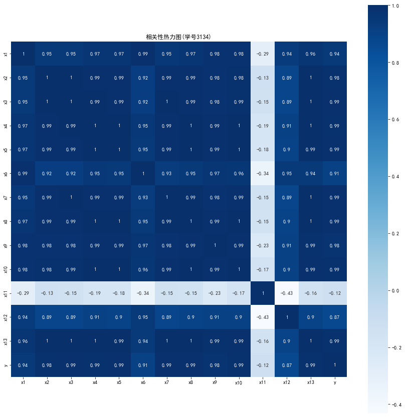
相关系数矩阵:
        x1    x2    x3    x4    x5    x6    x7    x8    x9   x10   x11   x12  \
x1   1.00  0.95  0.95  0.97  0.97  0.99  0.95  0.97  0.98  0.98 -0.29  0.94
x2   0.95  1.00  1.00  0.99  0.99  0.92  0.99  0.99  0.98  0.98 -0.13  0.89
x3   0.95  1.00  1.00  0.99  0.99  0.92  1.00  0.99  0.98  0.99 -0.15  0.89
x4   0.97  0.99  0.99  1.00  1.00  0.95  0.99  1.00  0.99  1.00 -0.19  0.91
x5   0.97  0.99  0.99  1.00  1.00  0.95  0.99  1.00  0.99  1.00 -0.18  0.90
x6   0.99  0.92  0.92  0.95  0.95  1.00  0.93  0.95  0.97  0.96 -0.34  0.95
x7   0.95  0.99  1.00  0.99  0.99  0.93  1.00  0.99  0.98  0.99 -0.15  0.89
x8   0.97  0.99  0.99  1.00  1.00  0.95  0.99  1.00  0.99  1.00 -0.15  0.90
x9   0.98  0.98  0.98  0.99  0.99  0.97  0.98  0.99  1.00  0.99 -0.23  0.91
x10  0.98  0.98  0.99  1.00  1.00  0.96  0.99  1.00  0.99  1.00 -0.17  0.90
x11 -0.29 -0.13 -0.15 -0.19 -0.18 -0.34 -0.15 -0.15 -0.23 -0.17  1.00 -0.43
x12  0.94  0.89  0.89  0.91  0.90  0.95  0.89  0.90  0.91  0.90 -0.43  1.00
x13  0.96  1.00  1.00  1.00  0.99  0.94  1.00  1.00  0.99  0.99 -0.16  0.90
y    0.94  0.98  0.99  0.99  0.99  0.91  0.99  0.99  0.98  0.99 -0.12  0.87

      x13     y
x1   0.96  0.94
x2   1.00  0.98
x3   1.00  0.99
x4   1.00  0.99
x5   0.99  0.99
x6   0.94  0.91
x7   1.00  0.99
x8   1.00  0.99
x9   0.99  0.98
x10  0.99  0.99
x11 -0.16 -0.12
x12  0.90  0.87
x13  1.00  0.99
y    0.99  1.00
相关性热力图:
import matplotlib.pyplot as plt
import seaborn as sns
plt.subplots(figsize=(15,15)) #设置画面大小
sns.heatmap(corr,annot=True,vmax=1,square=True,cmap="Blues")
plt.rcParams['font.sans-serif'] = ['SimHei'] # 添加这条可以让图形显示中文
plt.rcParams['axes.unicode_minus'] = False # 添加这条可以让图形显示负号
plt.title('相关性热力图(学号3134)')
plt.show()
plt.close
<function matplotlib.pyplot.close(fig=None)>
import numpy as np
import pandas as pd
from sklearn.linear_model import Lasso
inputfile = "D:/Jupyter/a/data.csv"
data = pd.read_csv(inputfile) #读取数据
lasso = Lasso(1000) #调用Lasso()函数,设置λ的值为1000
lasso.fit(data.iloc[:,0:13],data['y'])
print('相关系数为:',np.round(lasso.coef_,5)) #输出结果,保留五位小数
print('相关系数非零个数为:',np.sum(lasso.coef_ !=0)) #计算相关系数非零的个数
mask = lasso.coef_ !=0 #返回一个相关系数是否为零的布尔数组
mask = np.append(mask,True) #将mask的元素补齐到14个
print('相关系数是否为零:',mask)
outputfile = "D:/Jupyter/a/new_reg_data.csv" #输出的数据文件
new_reg_data = data.iloc[:,mask] #返回相关系数非零的数据
new_reg_data.to_csv(outputfile) #存储数据
print('输出数据的维度为:',new_reg_data.shape) #查出输出数据的维度
相关系数为: [-1.8000e-04 -0.0000e+00  1.2414e-01 -1.0310e-02  6.5400e-02  1.2000e-04
  3.1741e-01  3.4900e-02 -0.0000e+00  0.0000e+00  0.0000e+00  0.0000e+00
 -4.0300e-02]
相关系数非零个数为: 8
相关系数是否为零: [ True False  True  True  True  True  True  True False False False False
  True  True]
输出数据的维度为: (20, 9)


GM11灰色预测:
import sys
sys.path.append("D:/Jupyter/a/GM11.py")
import numpy as np
import pandas as pd
from GM11 import GM11 #引入自编的灰色预测函数
inputfile1 = "D:/Jupyter/a/new_reg_data.csv"
inputfile2 = "D:/Jupyter/a/data.csv"
new_reg_data = pd.read_csv(inputfile1) #读取经过属性选择后的数据
data = pd.read_csv(inputfile2) #读取总的数据
new_reg_data.index = range(1994,2014)
new_reg_data.loc[2014] = None
new_reg_data.loc[2015] = None
cols = ['x1','x3','x4','x5','x6','x7','x8','x13']
for i in cols:
f = GM11(new_reg_data.loc[range(1994, 2014),i].values)[0]
new_reg_data.loc[2014,i] = f(len(new_reg_data)-1) #2014年预测结果
new_reg_data.loc[2015,i] = f(len(new_reg_data)) #2015年预测结果
new_reg_data[i] = new_reg_data[i].round(2) #保留两位小数
outputfile = ("D:/Jupyter/a/new_reg_data_GM11.xls") #灰色预测后保存的路径
y = list(data['y'].values) #提取财政收入列,合并至新数据框中
y.extend([np.nan,np.nan])
new_reg_data['y'] = y
new_reg_data.to_excel(outputfile) #结果输出
print('预测结果为:\n',new_reg_data.loc[2014:2015,:]) #预测展示
运行结果:
预测结果为:
Unnamed: 0 x1 x3 x4 x5 x6 \
2014 NaN 8142148.24 7042.31 43611.84 35046.63 8505522.58
2015 NaN 8460489.28 8166.92 47792.22 38384.22 8627139.31
x7 x8 x13 y
2014 4600.40 18686.28 44506.47 NaN
2015 5214.78 21474.47 49945.88 NaN
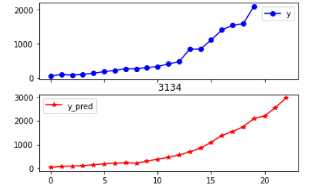
读取真实值和预测值以及绘图:
import numpy as np
import pandas as pd
import matplotlib.pyplot as plt
from sklearn.svm import LinearSVR
inputfile = "D:/Jupyter/a/new_reg_data_GM11.xls" # 灰色预测后保存的路径
data = pd.read_excel(inputfile) # 读取数据
feature = ['x1', 'x3', 'x4', 'x5', 'x6', 'x7', 'x8', 'x13'] # 属性所在列
data.index = range(1994, 2016)
data_train = data.loc[range(1994, 2014)].copy() # 取2014年前的数据建模
data_mean = data_train.mean()
data_std = data_train.std()
data_train = (data_train - data_mean)/data_std # 数据标准化
x_train = data_train[feature].to_numpy() # 属性数据
y_train = data_train['y'].to_numpy() # 标签数据
linearsvr = LinearSVR() # 调用LinearSVR()函数
linearsvr.fit(x_train,y_train)
x = ((data[feature] - data_mean[feature])/data_std[feature]).to_numpy() # 预测,并还原结果。
data['y_pred'] = linearsvr.predict(x) * data_std['y'] + data_mean['y']
outputfile ="D:/Jupyter/a/new_reg_data_GM11_revenue.xls" # SVR预测后保存的结果
data.to_excel(outputfile)
print('真实值与预测值分别为:\n',data[['y','y_pred']])
fig = data[['y','y_pred']].plot(subplots = True, style=['b-o','r-*']) # 画出预测结果图
plt.rcParams['font.sans-serif'] = ['SimHei'] # 添加这条可以让图形显示中文
plt.title('学号3134')
plt.show()
运行结果:
真实值与预测值分别为:
             y       y_pred
1994    64.87    36.398159
1995    99.75    83.087398
1996    88.11    93.932645
1997   106.07   105.688993
1998   137.32   150.374784
1999   188.14   187.547478
2000   219.91   219.023937
2001   271.91   229.813319
2002   269.10   219.160152
2003   300.55   300.150491
2004   338.45   383.247124
2005   408.86   463.134719
2006   476.72   554.969405
2007   838.99   691.722453
2008   843.14   843.602663
2009  1107.67  1088.925561
2010  1399.16  1380.766418
2011  1535.14  1538.342397
2012  1579.68  1740.991244
2013  2088.14  2088.140000
2014      NaN  2190.565775
2015      NaN  2542.166255

 浙公网安备 33010602011771号