

Matlab——m_map指南(3)——实例
m_map 实例
1、
clear all
m_proj('ortho','lat', 48,'long',-123');%投影方式,范围
m_coast('patch','r');%红色填充
m_grid('linest','-','xticklabels',[],'yticklabels',[]);%标注为空
patch(.55*[-1 1 1 -1],.25*[-1 -1 1 1]-.55,'w');%四个点,白色填充
text(0,-.55,'M\_Map','fontsize',25,'color','b',...
   'vertical','middle','horizontal','center');%填充内容,属性要求,垂直水平居中,斜杠转义符
set(gcf,'units','inches','position',[2 2 3 3]);%设置图片大小
set(gcf,'paperposition',[3 16 6 6]);%[left bottom width height].

2.
clear all
m_proj('lambert','long',[-160 -40],'lat',[30 80]);
m_coast('patch',[1 .85 .7]);%填充海岸线
m_elev('contourf',[500:500:6000]);%海深等高线
m_grid('box','fancy','tickdir','in');
colormap(flipud(copper));%翻转三原色的顺序排列,重新画图
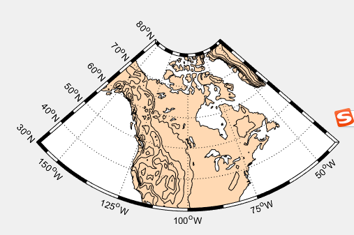
3、
m_proj('stereographic','lat',90,'long',30,'radius',25);
m_elev('contour',[-3500:1000:-500],'edgecolor','b');
m_grid('xtick',12,'tickdir','out','ytick',[70 80],'linest','-');
m_coast('patch',[.7 .7 .7],'edgecolor','r');

4、
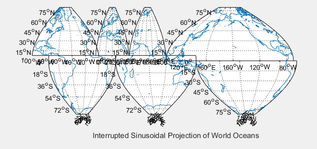
4.1默认的加载形式
clear all
Slongs=[-100 0;-75 25;-5 45; 25 145;45 100;145 295;100 290];
Slats= [  8 80;-80  8; 8 80;-80   8; 8  80;-80   0;  0  80];
for l=1:7,
 m_proj('sinusoidal','long',Slongs(l,:),'lat',Slats(l,:));%分区块的载入地图
 m_grid;
 m_coast;
end;
xlabel('Interrupted Sinusoidal Projection of World Oceans');
% In order to see all the maps we must undo the axis limits set by m_grid calls:
set(gca,'xlimmode','auto','ylimmode','auto');%自动加载所有数据
4.2
clear all
subplot(211);
Slongs=[-100 0;-75 25;-5 45; 25 145;45 100;145 295;100 290];
Slats= [  8 80;-80  8; 8 80;-80   8; 8  80;-80   0;  0  80];
for l=1:7,
 m_proj('sinusoidal','long',Slongs(l,:),'lat',Slats(l,:));
 m_grid('fontsize',6,'xticklabels',[],'xtick',[-180:30:360],...%字体尺寸,隐藏坐标,坐标等距离排列
        'ytick',[-80:20:80],'yticklabels',[],'linest','-','color',[.9 .9 .9]);%线条形式实线,颜色
 m_coast('patch','g');%填充绿色
end;
xlabel('Interrupted Sinusoidal Projection of World Oceans');
% In order to see all the maps we must undo the axis limits set by m_grid calls:
set(gca,'xlimmode','auto','ylimmode','auto');

subplot(212);
Slongs=[-100 43;-75 20; 20 145;43 100;145 295;100 295];
Slats= [  0  90;-90  0;-90   0; 0  90;-90   0;  0  90];%比上面范围重叠更多
for l=1:6,
 m_proj('mollweide','long',Slongs(l,:),'lat',Slats(l,:));
 m_grid('fontsize',6,'xticklabels',[],'xtick',[-180:30:360],...
        'ytick',[-80:20:80],'yticklabels',[],'linest','-','color','k');
 m_coast('patch',[.6 .6 .6]);
end;
xlabel('Interrupted Mollweide Projection of World Oceans');
set(gca,'xlimmode','auto','ylimmode','auto');%自动加载所有数据范围

5、
clear all
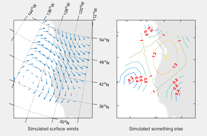
% Nice looking data
[lon,lat]=meshgrid([-136:2:-114],[36:2:54]);
u=sin(lat/6);%?
v=sin(lon/6);
m_proj('oblique','lat',[56 30],'lon',[-132 -120],'aspect',.8);%注意纬度顺序,高纬到低纬,'aspect'长宽比
subplot(121);
m_coast('patch',[.9 .9 .9],'edgecolor','none');
m_grid('tickdir','out','yaxislocation','right',...%边缘经纬线在外,纬度在右,经度在顶
'xaxislocation','top','xlabeldir','end','ticklen',.05);%边缘经纬度宽度
hold on;%图层合并
m_quiver(lon,lat,u,v);%经度,纬度,向东,向北的速度分量,转化为矢量箭头
xlabel('Simulated surface winds');
subplot(122);
m_coast('patch',[.9 .9 .9],'edgecolor','none');
m_grid('tickdir','in','yticklabels',[],...
'xticklabels',[],'linestyle','none','ticklen',.02);%经纬线去除
hold on;
[cs,h]=m_contour(lon,lat,sqrt(u.*u+v.*v));%画出轮廓
clabel(cs,h,'fontsize',10,'Color','red','FontWeight','bold');%标注轮廓,字体,字体大小,颜色
xlabel('Simulated something else');
6、
clear all
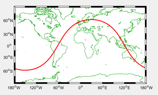
% Plot a circular orbit
lon=[-180:180];
lat=atan(tan(60*pi/180)*cos((lon-30)*pi/180))*180/pi;
m_proj('miller','lat',80);%查询,纬度(-80 80),经度(-180 180)
m_coast('color',[0 .6 0]);
m_line(lon,lat,'linewi',2,'color','r');%线宽,2;颜色
m_grid('linestyle','none','box','fancy','tickdir','in');%没有网格,边框相间,
%m_line(lon,lat,'linewi',2,'color','r','linestyle',':');控制线条格式,点画线还是直线
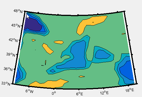
7、
clear all
m_proj('lambert','lon',[-10 20],'lat',[33 48]);%范围设置与投影有关系
m_tbase('contourf');%画5-min数据库轮廓
m_grid('linestyle','none','tickdir','out','linewidth',3);
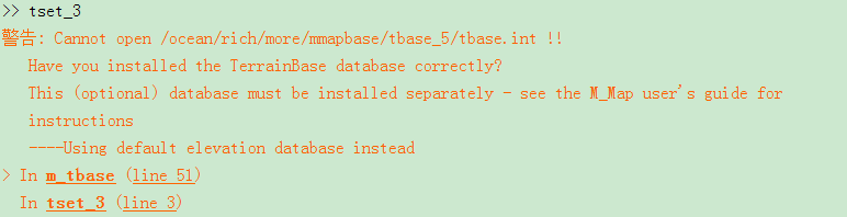
没有安装terrainbase,所以轮廓很简陋,这个坑用到的时候再填
8、不同分辨率情况下画的图
clear all
% Example showing the default coastline and all of the different resolutions
% of GSHHS coastlines as we zoom in on a section of Prince Edward Island.

clf
axes('position',[0.35 0.6 .37 .37]);%[left  bottom  width  height]
m_proj('albers equal-area','lat',[40 60],'long',[-90 -50],'rect','on');%方形,扇形
m_coast('patch',[0 1 0]);%填充
m_grid('linest','none','linewidth',2,'tickdir','out','xaxisloc','top','yaxisloc','right');
m_text(-69,41,'Standard coastline','color','r','fontweight','bold');%经纬度,内容,格式

axes('position',[.09 .5 .37 .37]);
m_proj('albers equal-area','lat',[40 54],'long',[-80 -55],'rect','on');
m_gshhs_c('patch',[.2 .8 .2]);
m_grid('linest','none','linewidth',2,'tickdir','out','xaxisloc','top');
m_text(-80,52.5,'GSHHS\_C (crude)','color','m','fontweight','bold','fontsize',14);

axes('position',[.13 .2 .37 .37]);
m_proj('albers equal-area','lat',[43 48],'long',[-67 -59],'rect','on');
m_gshhs_l('patch',[.4 .6 .4]);
m_grid('linest','none','linewidth',2,'tickdir','out');
m_text(-66.5,43.5,'GSHHS\_L (low)','color','m','fontweight','bold','fontsize',14);

axes('position',[.35 .05 .37 .37]);
m_proj('albers equal-area','lat',[45.8 47.2],'long',[-64.5 -62],'rect','on');
m_gshhs_i('patch',[.5 .6 .5]);
m_grid('linest','none','linewidth',2,'tickdir','out','yaxisloc','right');
m_text(-64.4,45.9,'GSHHS\_I (intermediate)','color','m','fontweight','bold','fontsize',14);

axes('position',[.55 .23 .37 .37]);
m_proj('albers equal-area','lat',[46.375 46.6],'long',[-64.2 -63.7],'rect','on');
m_gshhs_h('patch',[.6 .6 .6]);
m_grid('linest','none','linewidth',2,'tickdir','out','xaxisloc','top','yaxisloc','right');
m_text(-64.18,46.58,'GSHHS\_H (high)','color','m','fontweight','bold','fontsize',14);
运行出现这样问题
网站https://www.ngdc.noaa.gov/mgg/shorelines/data/gshhs/oldversions/version1.10/下载

下载version1.10中 gshhs_1.10.zip 文件,将zip文件解压,把gshhs_*.b 文件复制到 matlab\R2009\toolbox\matlab\m_map\@private 文件夹内。打开m_gshhs_c.m,补全路径。
FILNAME='D:\MATLAB\toolbox\m_map\private/gshhs_c.b'
同理将所有的m_gshhs_*.m路径都补充完整。

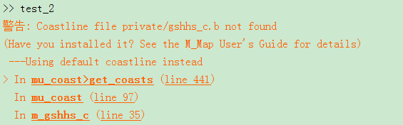
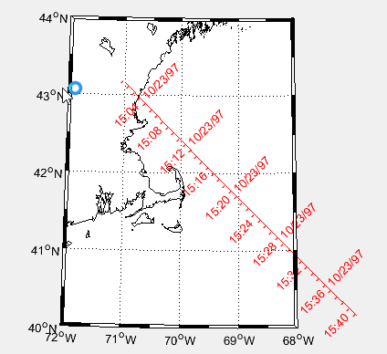
9、
clear all
m_proj('UTM','long',[-72 -68],'lat',[40 44]);
m_gshhs_i('color','k');
m_grid('box','fancy','tickdir','in');

% fake up a trackline
lons=[-71:.1:-67];
lats=60*cos((lons+115)*pi/180);%轨迹经纬度
dates=datenum(1997,10,23,15,1:41,zeros(1,41));%轨迹时间,1分钟到41分钟

m_track(lons,lats,dates,'ticks',0,'times',4,'dates',8,...%刻度间隔,时间间隔4分钟,日期标签间隔8分钟
        'clip','off','color','r','orient','upright');%颜色标签方向
10、范围环
clear all
m_proj('hammer','clong',170);%缩放范围
m_grid('xtick',[],'ytick',[],'linestyle','-');
m_coast('patch','g');
m_line(100.5,13.5,'marker','square','color','r');%增加了一个标记点
m_range_ring(100.5,13.5,[1000:1000:15000],'color','b','linewi',2);%范围,颜色,线宽
xlabel('1000km range rings from Bangkok');%曼谷中心1000km的范围环

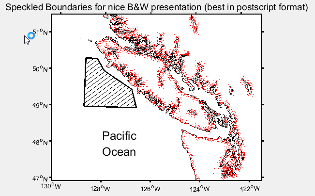
11、
clear all
bndry_lon=[-128.8 -128.8 -128.3 -128 -126.8 -126.6 -128.8];
bndry_lat=[  49    50.33  50.33  50   49.5   49     49];

clf;
m_proj('lambert','long',[-130 -121.5],'lat',[47 51.5],'rectbox','on');

m_gshhs_i('color','k');              % Coastline...
m_gshhs_i('speckle','color','r');    % with speckle added,斑点添加

m_line(bndry_lon,bndry_lat,'linewi',2,'color','k');     % Area outline ...
m_hatch(bndry_lon,bndry_lat,'single',30,5,'color','k'); % ...with hatching added.斜线,30度,5个单位相距

m_grid('linewi',2,'linest','none','tickdir','out');
title('Speckled Boundaries for nice B&W presentation (best in postscript format)','fontsize',14);
m_text(-128,48,5,{'Pacific','Ocean'},'fontsize',18);
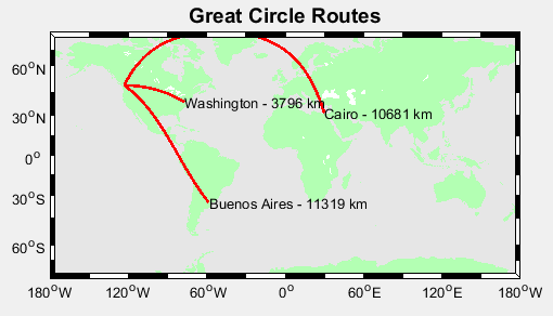
12
clear all

m_proj('miller','lat',[-75 75]);
m_coast('patch',[.7 1 .7],'edgecolor','none');
m_grid('box','fancy','linestyle','none','backcolor',[.9 .9 0.9]);

cities={'Cairo','Washington','Buenos Aires'};
lons=[ 30+2/60  -77-2/60   -58-22/60];
lats=[ 31+21/60  38+53/60  -34-45/60];

for k=1:3,
  [range,ln,lt]=m_lldist([-123-6/60 lons(k)],[49+13/60  lats(k)],40);
   %是两个位置之间分40个点,range返回距离,ln经度矩阵,lt纬度矩阵
  m_line(ln,lt,'color','r','linewi',2);
  m_text(ln(end),lt(end),sprintf('%s - %d km',cities{k},round(range)));
end;

title('Great Circle Routes','fontsize',14,'fontweight','bold');
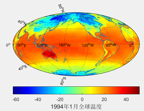
13、 全球/地区温度图
(1)读取数据
clear all
setup_nctoolbox %调用工具包
tic %计时
%%
nc=ncgeodataset('tmpsfc.gdas.199401.grb2'); %读文件
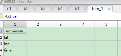
tem_1=nc.variables %浏览数据类型
%%
a1=nc.geovariable(tem_1(1));%取得数据类型为Temperature_surface的数据
b1=a1.data(1,:,:); %第一个时间点温度数据
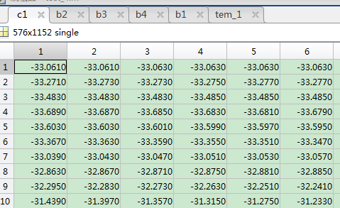
c1=squeeze(b1)-273.16;%删除单一维度,换为摄氏温度
%%
a2=nc.geovariable(tem_1(2));%取得数据类型为lat的数据,纬度
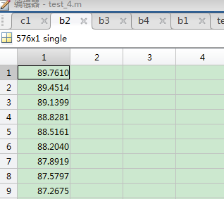
b2=a2.data(:,1)%提取数据
%%
a3=nc.geovariable(tem_1(3));%经度
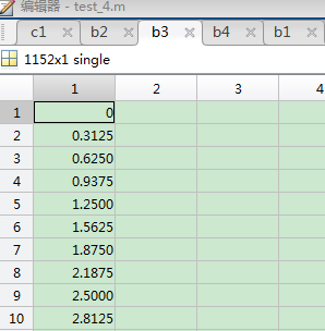
b3=a3.data(:,1)%
%%
a4=nc.geovariable(tem_1(4));%取得数据类型为time的数据
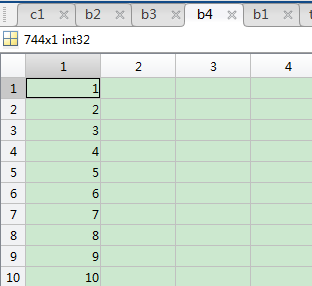
b4=a4.data(:,1)%
%%
save A b2 b3 c1
toc
读取的是NCEP/CFSR数据,1994年1月的温度数据。
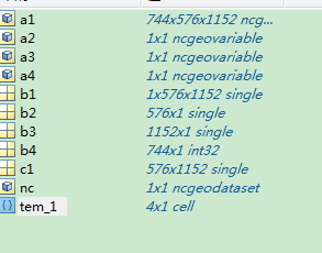
该数据一共四项。温度,纬度,经度,时间。
时间数据
经度数据
纬度数据
可以看出该数据集的数据组织形式,经度纬度构成世界地图,记录了744个时间点的温度数据。约等于1小时采集一次数据。
温度数据
保存为mat格式数据,为画图做准备。
(2)画图
clear all
load A

[Plg,Plt]=meshgrid(b3',b2');%形成网格

 m_proj('hammer-aitoff','clongitude',-150);%投影模式

m_pcolor(Plg,Plt,c1);
shading flat;
colormap('jet');%颜色选择
hold on;
m_pcolor(Plg-360,Plt,c1);
shading flat; %着色模式
colormap('jet');

m_coast();
m_grid('xaxis','middle');

% h=colorbar('h');
% set(get(h,'title'),'string','1991年1月全球温度');

c=colorbar('southoutside','fontsize',12)
c.Label.String = '1994年1月全球温度';
c.Label.FontSize = 15;
(3)找出最大、最小温度的经纬度
clear all
load C
Max_col=max(c1);%列最大值
Max_row=max(c1,[],2)%行最大值
Max=max(max(c1));
[x1,y1]=find(c1==max(max(c1)));%x 行,y 列
T_1=Plt(x1,y1)%纬度
T_2=Plg(x1,y1)%经度

Min_col=min(c1);%列最大值
Min_row=min(c1,[],2)%行最大值
Min=min(min(c1));
[x,y]=find(c1==min(min(c1)));%x 行,y 列
T_x=Plt(x,y)%纬度
T_y=Plg(x,y)%经度
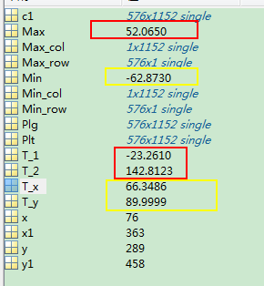
可以看出最热52度,在澳大利亚那块(142.8123E,23.2610S);最冷-62度,在北极圈那块(89.9999E,66.3486N)。
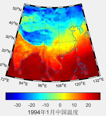
(4)中国(地区)温度图
clear all
load A
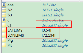
LATLIMS=[3 54];
LONLIMS=[72 134];%选定边界范围
[Plg,Plt]=meshgrid(b3',b2');%形成网格
m_proj('lambert','lon',LONLIMS,'lat',LATLIMS);%投影模式
m_pcolor(Plg,Plt,c1);
shading flat;
colormap('jet');%颜色选择
hold on;
m_pcolor(Plg-360,Plt,c1);
shading flat; %着色模式
colormap('jet');
m_coast();
m_grid('box','fancy','tickdir','in');
% h=colorbar('h');
% set(get(h,'title'),'string','1991年1月全球温度');
c=colorbar('southoutside','fontsize',12)
c.Label.String = '1994年1月中国温度';
c.Label.FontSize = 15;
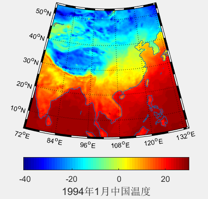
该方法是读取全球数据,只展示部分
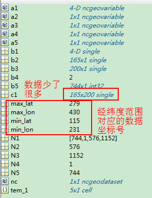
(5)
改进的区域方法,读取该区域的数据数据,
clear all
setup_nctoolbox %调用工具包
tic %计时
%%
min_lat=115;
max_lat=279;
min_lon=231;
max_lon=430;  %区域经纬度范围,在数据中的位置

%%
nc=ncgeodataset('tmp2m.gdas.199401.grb2');   %读文件
tem_1=nc.variables   %浏览数据类型
%%
N1=nc.size(tem_1(1));%读取数据大小,可以看出数据的组织形式
a1=nc.geovariable(tem_1(1));%取得数据类型为Temperature_surface的数据
b1=a1.data(1,1,min_lat:max_lat,min_lon:max_lon); %第一个时间点温度数据
c1=squeeze(b1)-273.16;%删除单一维度,换为摄氏温度
%%
N2=nc.size(tem_1(2));
a2=nc.geovariable(tem_1(2));%取得数据类型为lat的数据,纬度
b2=a2.data(min_lat:max_lat,1);%提取数据
%%
N3=nc.size(tem_1(3))
a3=nc.geovariable(tem_1(3));%经度
b3=a3.data(min_lon:max_lon,1);%
%%
N4=nc.size(tem_1(4))
a4=nc.geovariable(tem_1(4));%取得数据类型为time的数据
b4=a4.data(:,1);%
%%
N5=nc.size(tem_1(5));%读取数据大小
a5=nc.geovariable(tem_1(5));%取得数据类型为time的数据
b5=a5.data(:,1);%
%%
save tem b2 b3 c1
toc
clear all
load tem

LATLIMS=[3 54];
LONLIMS=[72 134];%选定边界范围

[Plg,Plt]=meshgrid(b3',b2');%形成网格

 m_proj('lambert','lon',LONLIMS,'lat',LATLIMS);%投影模式

m_pcolor(Plg,Plt,c1);
shading flat;
colormap('jet');%颜色选择
hold on;
m_pcolor(Plg-360,Plt,c1);
shading flat; %着色模式
colormap('jet');

m_coast();
m_grid('box','fancy','tickdir','in');

% h=colorbar('h');
% set(get(h,'title'),'string','1991年1月全球温度');

c=colorbar('southoutside','fontsize',12)
c.Label.String = '1994年1月中国温度';
c.Label.FontSize = 15;
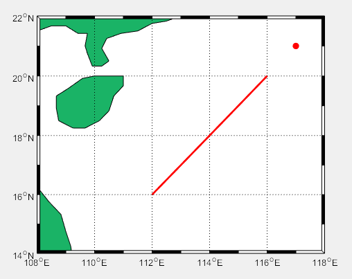
八、圆形区域的画图
1、
clear all

LATLIMS=[14 22];
LONLIMS=[108 118];%南海边界范围
m_proj('miller','lon',LONLIMS,'lat',LATLIMS);%投影模式
m_coast('patch',[0.1 0.7 0.4]);%绿色填充
m_grid('box','fancy','tickdir','in');%没有网格,边框相间,%m_line(lon,lat,'linewi',2,'color','r','linestyle',':');控制线条格式,点画线还是直线

lon=112:1:116;
lat=16:1:20;
m_line(lon,lat,'linewi',2,'color','r');%线宽,2;颜色

[X,Y]=m_ll2xy(117,21);
line(X,Y,'marker','.','markersize',24','color','r')%画点
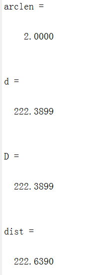
2、距离
clear all
%distance用法
arclen=distance([37,0],[35,0])%返回两点间的相对球心的角度,以度为单位
d=distance([37,0],[35,0],6371)% [纬度,经度] [纬度,经度] [半径]
D=(arclen/180)*pi*6371
%m_map中函数
dist=m_lldist([0 0],[35 37])%[经度 经度] [纬度 纬度]
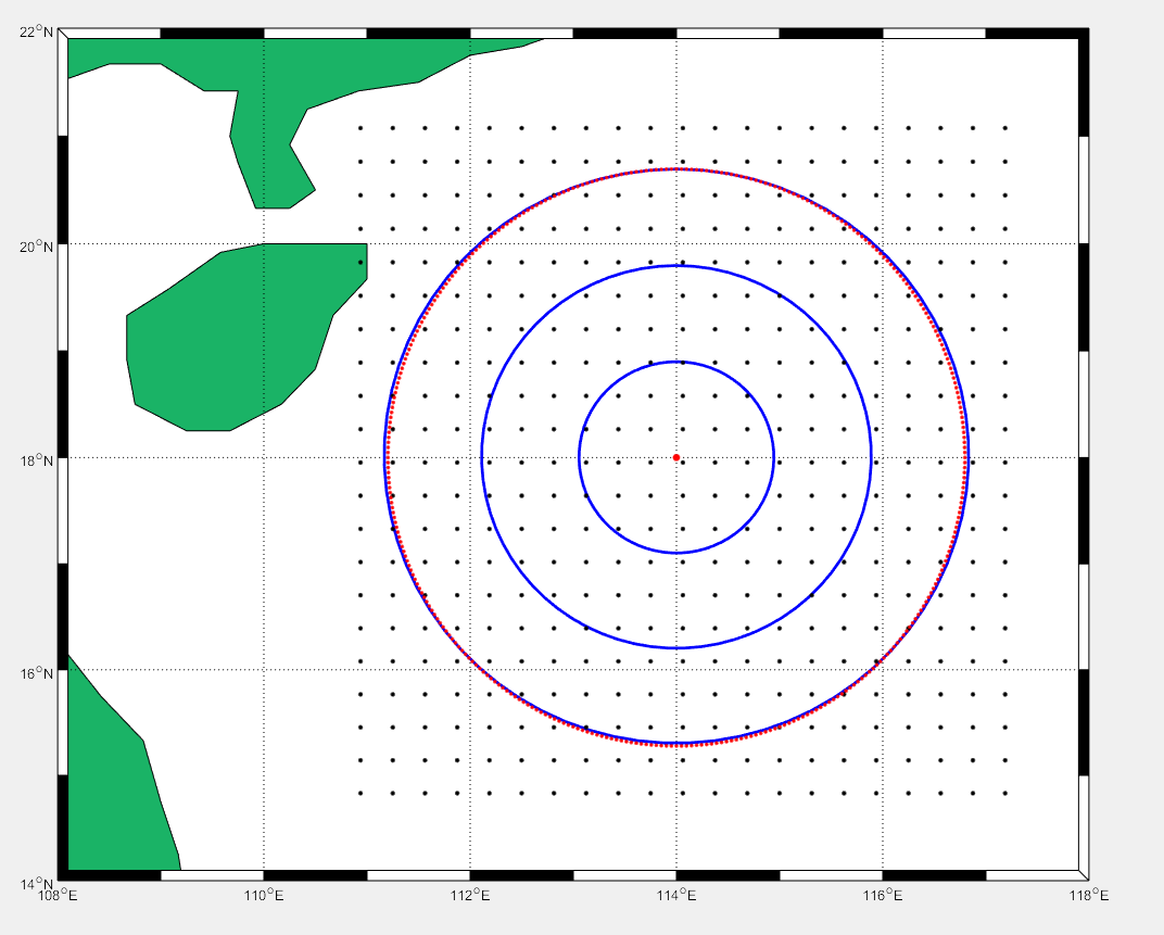
3、
clear all

LATLIMS=[14 22];
LONLIMS=[108 118];%南海边界范围
m_proj('miller','lon',LONLIMS,'lat',LATLIMS);%投影模式
m_coast('patch',[0.1 0.7 0.4]);%绿色填充
m_grid('box','fancy','tickdir','in');%没有网格,边框相间,%m_line(lon,lat,'linewi',2,'color','r','linestyle',':');控制线条格式,点画线还是直线

load EDH_south_sea_2008
load coordi_south_sea_2008

m_range_ring(114,18,[1e2:1e2:3e2],'linewi',2,'color','b');%红色300km范围圆圈

% 矩形点阵
range_lat=4:24;%21N和15N对应的位置下标
range_lon=20:40;%111.5E和116.5E对应的下标
for i=1:length(range_lon)
    for j=1:length(range_lat)
        [X,Y]=m_ll2xy(lon_south_sea(range_lon(i)),lat_south_sea(range_lat(j)));%化为x,y坐标
        line(X,Y,'marker','.','markersize',10,'color','k')%画点
        hold on
    end
end

%离散圆
[X0,Y0]=m_ll2xy(114,18);%化为x,y坐标
line(X0,Y0,'marker','.','markersize',15,'color','r');%画圆心
DIST=m_lldist([114 114],[18 19]);%纬度加1度,增加的距离
R=300;%300km
[X1,Y1]=m_ll2xy(114,18+R/DIST);%找到300km的一个点

r=sqrt((X0-X1)^2+(Y0-Y1)^2);%地图距离到图上距离转换
theta=0:pi/180:2*pi;%360度,360个点。
x=X0+r*cos(theta); %(X0,Y0)圆心
y=Y0+r*sin(theta);
plot(x,y,'.','color','r')
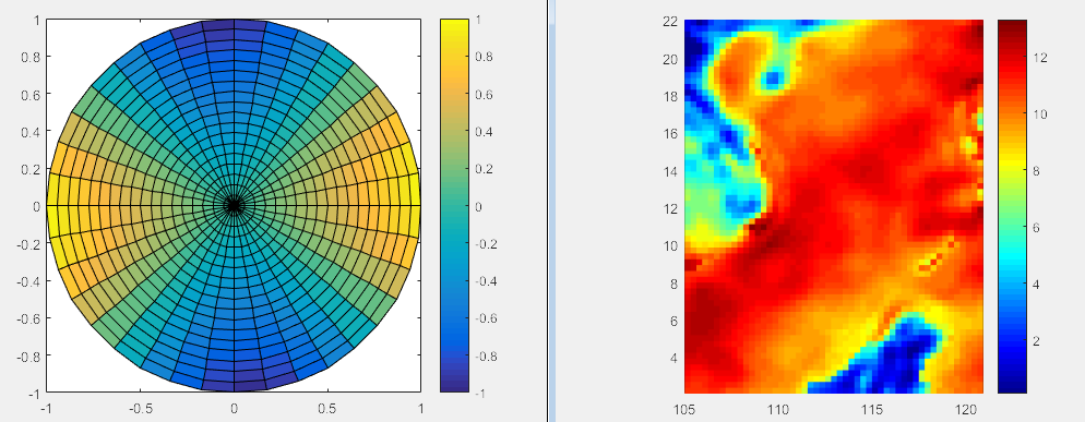
4、pcolor
clear all
n =18;
r = (0:n)'/n;
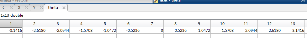
theta = pi*(-n:n)/n;
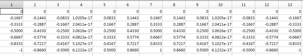
X = r*cos(theta);
Y = r*sin(theta);
C = r*cos(2*theta);
pcolor(X,Y,C)
axis equal tight
colorbar
figure
load PCOLOR %南海坐标和波导高度数据
colormap('jet');
shading flat;%平滑方式
gca=pcolor(Plg,Plt,EDH_south_sea)
set(gca, 'LineStyle','none');%去除网格
axis equal tight %按比例展示
colorbar %颜色条
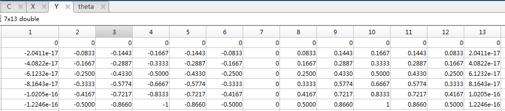
clear all
n =6;
r = (0:n)'/n;%0到6,半径上均分的数
theta = pi*(-n:n)/n;%将整个圆分成了13分。
X = r*cos(theta);
Y = r*sin(theta);
C = r*cos(2*theta);
pcolor(X,Y,C)
axis equal tight
colorbar

 浙公网安备 33010602011771号