LQR Controller

Assume that we have a linear system which is given by the following equation:
\begin{equation}
\dot{x} = Ax + Bu \
y = Cx + Du
\end{equation}

And we define a cost function
\begin{equation}
J = \frac{1}{2}\int_0^{T} (x^TQx+uTRu)dt
\end{equation}

There are two approaches to address this problem, namely: maximum principle and alternative one.

Approaches

• Maximum principle, this can be found at any textbook.
• Alternative one,
  For control purpose, we need to design a control input \(u=-Kx\) which can make the system performance reach our requirements. If we put this control input into your state-space equation, then it becomes

  $$	  \dot{x} = (A-BK)x = A_cx$$
  For the open-loop system, the poles of system is the eigenvalue of matrix $A$. For the close-loop system, state-space matrix $A$ becomes $A-BK$, which means we can determine values of $K$ to let poles of close-loop system to be required. Here, we need to point out that there is no relationship between $C,D$ when designing controller.
  Substituting $u=-Kx$ into cost function, it becomes 
  $$J=J = \frac{1}{2}\int_0^{T} x^T(Q+K^TRK)x dt$$
  in order to found $K$, we assume that there exists one constant matrix $P$ which statisfy
  $$\frac{d}{dt}(x^TPx)=-x^T(Q+K^TRK)x$$
  Put this equation into $J$ and expanse above equation, we get 
  ![enter image description here](http://mmbiz.qpic.cn/mmbiz_png/O60Uib8kfuu981V1E67WWibZMQhqROiarLnBsibHsscZuqISPzfKmkHzfErGibFgVbAJv0ESICD182zerZGueLtfLag/640?wx_fmt=png&tp=webp&wxfrom=5&wx_lazy=1)
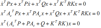
  Let $K=R^{-1}B^TP$, then
  ![enter image description here](http://mmbiz.qpic.cn/mmbiz_png/O60Uib8kfuu981V1E67WWibZMQhqROiarLnicuI5Tmo4ze0LCRiaX1PTpzP1AiaRwM4bFDOBjJnE1ItHJb6NAupOb6Ag/640?wx_fmt=png&tp=webp&wxfrom=5&wx_lazy=1)

Conclusion:

1. chose parameter \(Q,R\)
2. Compute Riccati equation and obtain \(P\).
3. Compute \(K=R^{-1}B^TP\). In matlab, it is K = lqr(A,B,Q,R);

===========
Example 1:
A=[0 1 0 0; 0 0 -1 0; 0 0 0 1; 0 0 9 0];
B = [0; 0.1; 0 ; -0.1];
C = [0 0 1 0];
D = 0;
Q = eye(4); R = 0.1;
K = lqr(A,B,Q,R);
Ac = A-B*K;
x0 = [0.1;0;0.1;0];
t = 0:0.05:20;
u = zeros(size(t));
[y,x] = lsim(Ac,B,C,D,u,t,x0);
plot(x,y)

State feedback with reference trajectory

Problem statement: Suppose that we are given a system \(\dot{x}=f(x,u)\) and a feasible trajectory \((x_d, u_d)\) . We wish to design a compensator of the form \(u=\alpha(x,x_d,u_d)\) such that \(lim_{t\to\infty}x-x_d =0\) . This is known as the trajectory tracking problem.
To design the controller, we construct the error system. We will assume for simplicity that \(f(x,u)=f(x)+g(x)u\). Let \(e=x-x_d,v=u-u_d\) and compute the dynamics for the error:

\[\dot{e}=\dot{x}-\dot{x_d}=f(e+x_d)-f(x_d)+g(e+x_d)(v+u_d)-g(x_d)u_d\\=F(e,v,x_d(t),u_d(t)) \]

In general, this system is time varying.
For trajectory tracking, we can assume that e is small and we can linearize around \(e=0\):

\[\dot{e}=A(t)e+B(t)v \]

where

\[A(t)=\frac{\partial F}{\partial e}|_(x_d(t),u_d(t), B(t)=\frac{\partial F}{\partial v}|_(x_d(t),u_d(t) \]

It is often the case that A(t) and B(t) depend only on \(x_d\), in which case it is convenient to write \(A(t)=A(x_d), B(t)=B(x_d)\).
If we design a state feedback control $K(x_d) $ for each \(x_d\), then we can regulate the system using

\[v=-K(x_d)e. \]

Substituting back the definitions of \(e,v\), our controller becomes

\[u=-K(x_d)(x-x_d)+u_d \]

In the special case of a linear system, it is easy to see that the error dynamics are identical to the system dynamics \(\dot{e}=Ae+Bv\) and in this case we don't need to schedule the gain based on \(x_d\), we can simply compute a constant gain \(K\) and write

\[u=-K(x-x_d)+u_d \]

Above equation is just useful for perfect model. However, there must be some uncertainties. An alternative to calibration is to make use of integral feedback, in which the controller uses an integrator to provide zero steady state error. We do this by augmenting the description of the system with a new state \(z\):
\(\frac{d}{dt}[x;z]=[Ax+Bu;y-r]=[Ax+Bu;Cx-r]\)
the compensator can be given by:

\[u=-K(x-x_e)-K_iz+u_d,\dot{z}=y-r \]

where \(x_e=-(A-BK)^{-1}B(u_d-K_iz_e)\)
Reference 1