1. 一阶系统微分方程
典型一阶系统微分方程
\[\frac{dx(t)}{dt}+ax(t)=au(t)
\]
零初始条件 \(x(0)=u(0)=0\) ,对其进行拉普拉斯变换
\[sX(s)+aX(s)=aU(s)
\]
调整得到传递函数
\[G(s)=\frac{X(s)}{U(s)}=\frac{a}{s+a}
\]
单位冲激函数
\[\left\{
\begin{array}{lc}
\delta(t)=0,t\neq 0 \\
\int^\infty _{-\infty} \delta(t)dt=1
\end{array}
\right.
\]
\[\mathcal{L}[\delta(t)]=\int_{0}^{\infty}\delta(t) \mathrm{e}^{-st} \mathrm{d}t=\mathrm{e}^{-s0}=1
\]
单位阶跃函数
\[u\left(t\right)=\begin{cases}1,&t\geqslant0\\\\0,&t<0\end{cases}
\]
\[\mathcal{L}[1]=\mathcal{L}[\mathrm{e}^{-0t}]=\frac{1}{s+0}=\frac{1}{s}
\]
2.一阶系统冲激响应
当系统的输入为单位冲激函数时,\(u(t)=\delta(t),U(s)=1\),代入得
\[X(s)=U(s)G(s)=1\times\frac{a}{s+a}=\frac{a}{s+a}
\]
逆变换为
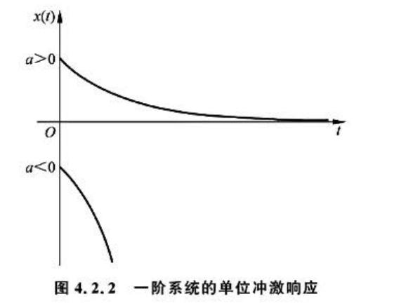
\[x\left(t\right)=\mathcal{L}^{-1}\left[X\left(s\right)\right]=\mathcal{L}^{-1}\left[\frac{a}{s+a}\right]=a \mathrm{e}^{-at}
\]
![image]()
图显示 了一阶系统在 不同 值 下的单 位冲激 响应。 可知当 单位冲 激输人 作用在一阶 系统时 ,系统 的输出x(t) 将从以a 开始 变化.
3.二阶系统一般形式
从一个典型的二阶系 统例子 人手, 一个弹 簧质量 阻尼系 统如图
\[m \frac{\mathrm{d}^{2}x\left(t\right)}{\mathrm{d}t^{2}}+b \frac{\mathrm{d}x\left(t\right)}{\mathrm{d}t}+kx\left(t\right)=f\left(t\right)\\
\]
调整可得
\[\frac{\mathrm{d}^{2}x\left(t\right)}{\mathrm{d}t^{2}}+\frac{b}{m} \frac{\mathrm{d}x\left(t\right)}{\mathrm{d}t}+\frac{k}{m}x\left(t\right)=\frac{1}{m}f\left(t\right)
\]
![image]()
固有频率或者自然频率 (Natural Frequency): \(\omega_{\mathrm{n}}=\sqrt{\frac{k}{m}}\)
阻尼比 ( Damping Ratio):\(\zeta=\frac b{2\sqrt{km}}。\)
代入得
\[\frac{\mathrm{d}^{2}x\left(t\right)}{\mathrm{d}t^{2}}+2\zeta\omega_{\mathrm{n}} \frac{\mathrm{d}x\left(t\right)}{\mathrm{d}t}+\omega_{\mathrm{n}}^{2}x\left(t\right)=\frac{1}{m}f\left(t\right)
\]
4.二阶系统传递函数
在本章中只讨论\(m>0,k>0,b>0\)的情况 ,因此\(\omega_\mathrm{n}>0\)且\(\zeta>0\)。其他例外情况读者可以根据本章的方法去处理。
考虑零初始状态,对式等号两边进行拉普拉斯变换并整理,可以得到一般形式二阶系统的传递函数,即
\[G(s)=\frac{X(s)}{U(s)}=\frac{\omega_{\mathrm{n}}^{2}}{s^{2}+2\zeta\omega_{\mathrm{n}}s+\omega_{\mathrm{n}}^{2}}
\]
5. 二阶系统状态空间
如果使用状态空间方程的表达形式,可以设系统的状态变量为\(z(t)=[z_1(t),z_2(t)]^\mathrm{T}=\begin{bmatrix}x\left(t\right),\frac{\mathrm{d}x\left(t\right)}{\mathrm{d}t}\end{bmatrix}^{\mathrm{T}}\)。
因为
\[\frac{\mathrm{d}^{2}x\left(t\right)}{\mathrm{d}t^{2}}=-2\zeta\omega_{\mathrm{n}} \frac{\mathrm{d}x\left(t\right)}{\mathrm{d}t}-\omega_{\mathrm{n}}^{2}x\left(t\right)+\frac{1}{m}f\left(t\right)
\]
而且 \(f(t)=u(t)k\),得到
\[\begin{aligned}&\frac{\mathrm{d}z_{1}\left(t\right)}{\mathrm{d}t}=z_{2}\left(t\right)\\&\frac{\mathrm{d}z_{2}\left(t\right)}{\mathrm{d}t}=\frac{\mathrm{d}^{2}z_{1}\left(t\right)}{\mathrm{d}t^{2}}=-2\zeta\omega_{\mathrm{n}}z_{2}\left(t\right)-\omega_{\mathrm{n}}^{2}z_{1}\left(t\right)+\omega_{\mathrm{n}}^{2}u\left(t\right)\end{aligned}
\]
写成矩阵形式
\[\begin{aligned}&\frac{\mathrm{d}z\left(t\right)}{\mathrm{d}t}=\mathbf{A}z\left(t\right)+\mathbf{B}u\left(t\right)
\end{aligned}
\]
其中
\[\begin{aligned}
&\mathbf{A}=\begin{bmatrix}0&1\\-\omega_\mathrm{n}^2&-2\zeta\omega_\mathrm{n}\end{bmatrix},\quad\mathbf{B}=\begin{bmatrix}0\\\omega_\mathrm{n}^2\end{bmatrix}\end{aligned}
\]
6. 二阶系统对初始状态的响应
当系统的输入 \(u(t)=0\) ,上式可以写成
\[\frac{\mathrm{d}z\left(t\right)}{\mathrm{d}t}=Az\left(t\right),\quad\text{其中}
\quad
\mathbf{A}=\begin{bmatrix}0&1\\-\omega_\mathrm{n}^2&-2\zeta\omega_\mathrm{n}\end{bmatrix}
\]
求系统的平衡点,令$ \frac{dz(t)}{dt}=0$ 可得
\[\begin{cases}
0=z_{2\mathrm{f}}
\\0=-\omega_{\mathrm{n}}^{2}z_{1\mathrm{f}}-2\zeta\omega_{\mathrm{n}}z_{2\mathrm{f}}\\
\end{cases}
\\
\Rightarrow
\begin{cases}z_{1\mathrm{f}}=0\\
z_{2\mathrm{f}}=0\end{cases}
\]
分析平 衡点的 性质, 首先要 得到状 态矩阵 A 的 特征值 ,令$|A-\lambda I |=0 $ 得到
\[\begin{vmatrix}-\lambda&1\\-\omega_\mathrm{n}^2&-2\zeta\omega_\mathrm{n}-\lambda\end{vmatrix}=\lambda^2+2\zeta\omega_\mathrm{n}\lambda+\omega_\mathrm{n}^2=0
\]
求解 特征值 ,得到
\[\begin{cases}\lambda_1=- \zeta\omega_\mathrm{n}+\omega_\mathrm{n}\sqrt{\zeta^2-1}\\\lambda_2=- \zeta\omega_\mathrm{n}-\omega_\mathrm{n}\sqrt{\zeta^2-1}\end{cases}
\]
特 征值$\lambda $ 对 应了传递函数G(s) 的 极点。
分类讨论不同的参数对特征值 \(\lambda_1\) 和$ \lambda_2$ 的影响,及特征值如何影响系统的稳定。


 浙公网安备 33010602011771号